9 OLS and Endogeneity
Just like many economic relationships are nonlinear, many economic variables are endogenous. By this we typically mean that \(X\) is an outcome determined (or caused: \(\to\)) by some other variable.
- If \(Y \to X\), then we have reverse causality
- If \(Y \to X\) and \(X \to Y\), then we have simultaneity
- If \(Z\to Y\) and either \(Z\to X\) or \(X \to Z\), then we have omitted a potentially important variable
These endogeneity issues imply \(X\) and \(\epsilon\) are correlated, which is a barrier to interpreting OLS as a causal model.
## Simulate data with an endogeneity issue
n <- 300
z <- rbinom(n,1,.5)
xy <- sapply(z, function(zi){
    y <- rnorm(1,zi,1)
    x <- rnorm(1,zi*2,1)
    c(x,y)
})
xy <- data.frame(x=xy[1,],y=xy[2,])
plot(y~x, data=xy, pch=16, col=grey(.5,.5))
abline(lm(y~x,data=xy))
With multiple linear regression, note that endogeneity biases are not just a problem your main variable. Suppose your interested in how \(x_{1}\) affects \(y\), conditional on \(x_{2}\). Letting \(X=[x_{1}, x_{2}]\), you estimate \[\begin{eqnarray} \hat{\beta}_{OLS} = [X'X]^{-1}X'y \end{eqnarray}\] You paid special attention in your research design to find a case where \(x_{1}\) is truly exogenous. Unfortunately, \(x_{2}\) is correlated with the error term. (How unfair, I know, especially after all that work). Nonetheless, \[\begin{eqnarray} \mathbb{E}[X'\epsilon] = \begin{bmatrix} 0 \\ \rho \end{bmatrix}\\ \mathbb{E}[ \hat{\beta}_{OLS} - \beta] = [X'X]^{-1} \begin{bmatrix} 0 \\ \rho \end{bmatrix} = \begin{bmatrix} \rho_{1} \\ \rho_{2} \end{bmatrix} \end{eqnarray}\] The magnitude of the bias for \(x_{1}\) thus depends on the correlations between \(x_{1}\) and \(x_{2}\) as well as \(x_{2}\) and \(\epsilon\).
Three statistical tools: 2SLS, RDD, and DID, are designed to address endogeneity issues. The elementary versions of these tools are linear regression. Because there are many textbooks and online notebooks that explain these methods at both high and low levels of technical detail, they are not covered extensively in this notebook. You are directed to the following resources which discuss these statistical models in more general terms and how they can be applied across many social sciences.
- Causal Inference for Statistics, Social, and Biomedical Sciences: An Introduction
- https://www.mostlyharmlesseconometrics.com/
- https://www.econometrics-with-r.org
- https://bookdown.org/paul/applied-causal-analysis/
- https://mixtape.scunning.com/
- https://theeffectbook.net/
- https://www.r-causal.org/
- https://matheusfacure.github.io/python-causality-handbook/landing-page.html
9.1 Two Stage Least Squares (2SLS)
There are many “Applied Statistics” approaches to 2SLS, and I encourage you to read up on them here
- https://www.econometrics-with-r.org/12-ivr.html
- https://bookdown.org/paul/applied-causal-analysis/estimation-2.html
- https://mixtape.scunning.com/07-instrumental_variables
- https://theeffectbook.net/ch-InstrumentalVariables.html
- http://www.urfie.net/read/index.html#page/247
I will focus on the seminal case in economics, which is complementary and hopefully provides much intuition
9.1.1 Competitive Market Equilibrium
Although there are many ways this simultaneity can happen, economic theorists have made great strides in analyzing the simultaneity problem as it arises from market relationships. In fact, the 2SLS statistical approach arose to understand the equilibrium of a single competitive market, which has three structural equations: (1) market supply is the sum of quantities supplied by individual firms, (2) market demand is the sum of quantities demanded by individual people, (3) market supply equals market demand. \[\begin{eqnarray} Q^{D}(P) &=& \sum_{i} q^{D}_{i}(P) \\ Q^{S}(P) &=& \sum_{i} q^{S}_{i}(P) \\ Q^{D} &=& Q^{S} = Q. \end{eqnarray}\] This last equation implies a simultaneous “reduced form” relationship where both the price and the quantity are outcomes. If there is a linear parametric structure to these equations, then you can examine how a change in parameters affects both price and quantity. Specifically, if \[\begin{eqnarray} \label{eqn:linear_demand} Q^{D}(P) &=& A^{D} - B^{D} P + \epsilon^{D},\\ \label{eqn:linear_supply} Q^{S}(P) &=& A^{S} + B^{S} P + \epsilon^{S}, \end{eqnarray}\] then equilibrium yields reduced form equations that collapse into intercept and residual terms; \[\begin{eqnarray} P^{*} &=& \frac{A^{D}-A^{S}}{B^{D}+B^{S}} + \frac{\epsilon^{D} - \epsilon^{S}}{B^{D}+B^{S}} = \alpha^{P} + \nu^{P}, \\ Q^{*} &=& \frac{A^{S}B^{D}+ A^{D}B^{S}}{B^{D}+B^{S}} + \frac{\epsilon^{S}B^{D}+ \epsilon^{D}B^{S}}{B^{D}+B^{S}}= \alpha^{Q} + \nu^{Q}. \end{eqnarray}\]
# Competitive Market Process

## Parameters
plm <- c(5,10) ## Price Range
P <- seq(plm[1],plm[2],by=.01) ## Price to Consider

## Demand Curve Simulator
qd_fun <- function(p, Ad=8, Bd=-.8, Ed_sigma=.25){
    Qd <- Ad + Bd*p + rnorm(1,0,Ed_sigma)
}

## Supply Curve Simulator
qs_fun <- function(p, As=-8, Bs=1, Es_sigma=.25){
    Qs <- As + Bs*p + rnorm(1,0,Es_sigma)
}
N <- 300 ## Number of Simulations
## Generate Equilibrium Data
## Plot Underlying Process
plot.new()
plot.window(xlim=c(0,2), ylim=plm)
EQ1 <- sapply(1:N, function(n){
## Market Mechanisms
demand <- qd_fun(P)
supply <- qs_fun(P)
## Compute EQ (what we observe)
eq_id <- which.min( abs(demand-supply) )
eq <- c(P=P[eq_id], Q=demand[eq_id])
## Plot Theoretical Supply and Demand behind EQ
lines(demand, P, col=grey(0,.01))
lines(supply, P, col=grey(0,.01))
points(eq[2], eq[1], col=grey(0,.05), pch=16)
## Return Equilibrium Observations
return(eq)
})
axis(1)
axis(2)
mtext('Quantity',1, line=2)
mtext('Price',2, line=2)
You can simply run a regression of one variable on another, but you will need much luck to correctly interrupt the resulting number. Consider regressing quantity on price; \[\begin{eqnarray} Q &=& \alpha^{Q} + \beta^{Q} P + \epsilon^{Q} = \alpha^{Q} + \beta^{Q} [\alpha^{P} + \beta^{P} Q + \epsilon^{P}] + \epsilon^{Q} \\ &=& \frac{[\alpha^{Q} + \epsilon^{Q}] + \beta^{Q} [\alpha^{P} + \epsilon^{P}]}{1-\beta^{P}} \end{eqnarray}\] We can see \(Q\) is a function of \(\epsilon^{P}\), thus biasing the estimate of \(\beta^{P}\). If you were to instead regress \(Q\) on \(P\), you would similarly get a number that is hard to interpret meaningfully. This simple derivation has a profound insight: price-quantity data does not generally tell you how price affects quantity supplied or demanded (and vice-versa).
## Analyze Market Data
dat1 <- data.frame(t(EQ1), cost='1')
reg1 <- lm(Q~P, data=dat1)
summary(reg1)
##
## Call:
## lm(formula = Q ~ P, data = dat1)
##
## Residuals:
## Min 1Q Median 3Q Max
## -0.57965 -0.11239 0.00777 0.12099 0.43285
##
## Coefficients:
## Estimate Std. Error t value Pr(>|t|)
## (Intercept) -0.62502 0.43661 -1.432 0.153326
## P 0.17010 0.04908 3.466 0.000606 ***
## ---
## Signif. codes: 0 '***' 0.001 '**' 0.01 '*' 0.05 '.' 0.1 ' ' 1
##
## Residual standard error: 0.1694 on 298 degrees of freedom
## Multiple R-squared: 0.03875, Adjusted R-squared: 0.03552
## F-statistic: 12.01 on 1 and 298 DF, p-value: 0.0006061If you have exogeneous variation on one side of the market, ``shocks’’, you can get information on the other. Experimental manipulation of \(A^{S}\) would, for example, allow you to trace out part of a demand curve: \[\begin{eqnarray} \frac{\partial P^{*}}{\partial A^{S}} = \frac{-1}{B^{D}+B^{S}}, \\ \frac{\partial Q^{*}}{\partial A^{S}} = \frac{B^{D}}{B^{D}+B^{S}}. \end{eqnarray}\] Notice that even in this linear model, all effects are conditional: The effect of a cost change on quantity or price depends on the demand curve. A change in costs affects quantity supplied but not quantity demanded (which then affects equilibrium price) but the demand side of the market still matters! The change in price from a change in costs depends on the elasticity of demand. (Likewise for changes in demand parameters.)
With two equations and two unknowns, we can estimate \(B^{D}\) and \(B^{S}\), which was the original idea behind 2SLS. Substituting the equilibrium condition into the structural demand equation, we can rewrite them as \[\begin{eqnarray} \label{eqn:linear_demand_iv} P(Q) &=& -\frac{A^{D}}{{B^{D}}} + \frac{Q^{s}}{B^{D}} - \frac{\epsilon^{D}}{B^{D}} = \alpha^{P} + \beta^{P} Q + \epsilon^{P}\\ \label{eqn:linear_supply_iv} Q(P) &=& A^{S} + \epsilon^{S} + B^{S} P . \end{eqnarray}\]
## Supply Shifter
EQ2 <- sapply(1:N, function(n){
    ## New Demand, but same par's
    demand <- qd_fun(P)
    ## New Supply Curves
    supply2 <- qs_fun(P, As=-6.5)
    ## lines(supply2, P, col=rgb(0,0,1,.01))
    ## Compute New EQ
    eq_id <- which.min( abs(demand-supply2) )
    eq <- c(P=P[eq_id], Q=demand[eq_id])
    #points(eq[2], eq[1], col=rgb(0,0,1,.05), pch=16)
    return(eq)
})

## Market Data w/ Supply Shift
dat2 <- data.frame(t(EQ2), cost='2')
dat2 <- rbind(dat1, dat2)


## Plot Market Data  w/ Supply Shift
cols <- ifelse(as.numeric(dat2$cost)==2, rgb(0,0,1,.2), rgb(0,0,0,.2))
plot.new()
plot.window(xlim=c(0,2), ylim=plm)
points(dat2$Q, dat2$P, col=cols, pch=16)
axis(1)
axis(2)
mtext('Quantity',1, line=2)
mtext('Price',2, line=2)
##
## Call:
## lm(formula = Q ~ P, data = dat2)
##
## Residuals:
##     Min      1Q  Median      3Q     Max
## -0.7649 -0.1575  0.0079  0.1575  0.7559
##
## Coefficients:
##             Estimate Std. Error t value Pr(>|t|)
## (Intercept)  6.67588    0.17781   37.55   <2e-16 ***
## P           -0.64312    0.02095  -30.69   <2e-16 ***
## ---
## Signif. codes:  0 '***' 0.001 '**' 0.01 '*' 0.05 '.' 0.1 ' ' 1
##
## Residual standard error: 0.2375 on 598 degrees of freedom
## Multiple R-squared:  0.6117, Adjusted R-squared:  0.611
## F-statistic:   942 on 1 and 598 DF,  p-value: < 2.2e-16
## Instrumental Variables Estimates
library(fixest)
reg2_iv <- feols(Q~1|P~cost, data=dat2)
summary(reg2_iv)## TSLS estimation, Dep. Var.: Q, Endo.: P, Instr.: cost
## Second stage: Dep. Var.: Q
## Observations: 600
## Standard-errors: IID
## Estimate Std. Error t value Pr(>|t|)
## (Intercept) 8.047036 0.204829 39.2867 < 2.2e-16 ***
## fit_P -0.804947 0.024145 -33.3384 < 2.2e-16 ***
## ---
## Signif. codes: 0 '***' 0.001 '**' 0.01 '*' 0.05 '.' 0.1 ' ' 1
## RMSE: 0.248603 Adj. R2: 0.572244
## F-test (1st stage), P: stat = 2,884.4, p < 2.2e-16, on 1 and 598 DoF.
## Wu-Hausman: stat = 553.5, p < 2.2e-16, on 1 and 597 DoF.If we had multiple alleged supply shifts and recorded their magnitudes, then we could recover more information about demand.
Caveat The coefficient interpretation rests on many assumptions. We have implicitly assumed
- both supply and demand are linear and additively seperable in covariates.
- only supply was affected, and it was only an intercept shift.
- the shock large enough to be picked up statistically.
We always get coefficients back when fitting feols but are rarely confident that all these assumptions hold. This is one reason why researchers often also report their OLS results.
9.2 Regression Discontinuities/Kink (RD/RK)
The basic idea here is to examine how a variable changes in response to an exogenous shock. Again, there is a large “Applied Statistics” literature I direct you to first
- https://bookdown.org/paul/applied-causal-analysis/rdd-regression-discontinuity-design.html
- https://mixtape.scunning.com/06-regression_discontinuity
- https://theeffectbook.net/ch-RegressionDiscontinuity.html
The Regression Discontinuities estimate of the cost shock is the difference in the outcome variable just before and just after the shock. We now turn to our canonical competitive market example. The RD estimate is the difference between the red and blue lines at \(T=300\).
dat2$T <- 1:nrow(dat2)

plot(P~T, dat2, main='Effect of Cost Shock on Price', pch=16, col=grey(0,.5))
regP1 <- lm(P~T, dat2[dat2$cost==1,])
lines(regP1$model$T, predict(regP1), col=2)
regP2 <- lm(P~T, dat2[dat2$cost==2,])
lines(regP2$model$T, predict(regP2), col=4)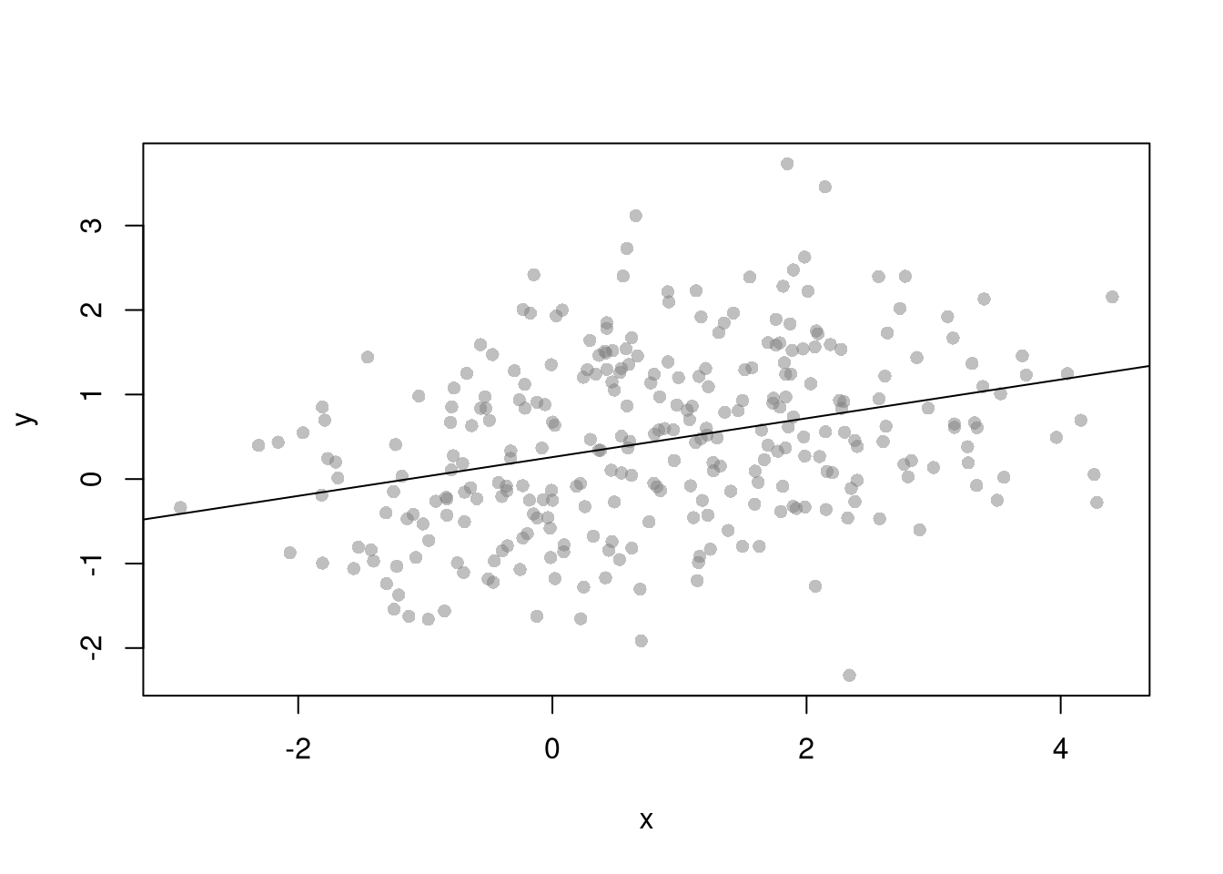
##
## Call:
## lm(formula = P ~ T * cost, data = dat2)
##
## Residuals:
##      Min       1Q   Median       3Q      Max
## -0.57978 -0.11984 -0.00214  0.12755  0.55403
##
## Coefficients:
##               Estimate Std. Error t value Pr(>|t|)
## (Intercept)  8.897e+00  2.227e-02 399.590   <2e-16 ***
## T           -2.265e-05  1.282e-04  -0.177    0.860
## cost2       -8.385e-01  6.290e-02 -13.331   <2e-16 ***
## T:cost2      7.149e-06  1.813e-04   0.039    0.969
## ---
## Signif. codes:  0 '***' 0.001 '**' 0.01 '*' 0.05 '.' 0.1 ' ' 1
##
## Residual standard error: 0.1923 on 596 degrees of freedom
## Multiple R-squared:  0.8283, Adjusted R-squared:  0.8274
## F-statistic: 958.3 on 3 and 596 DF, p-value: < 2.2e-16plot(Q~T, dat2, main='Effect of Cost Shock on Quantity', pch=16, col=grey(0,.5))
regQ1 <- lm(Q~T, dat2[dat2$cost==1,])
lines(regQ1$model$T, predict(regQ1), col=2)
regQ2 <- lm(Q~T, dat2[dat2$cost==2,])
lines(regQ2$model$T, predict(regQ2), col=4)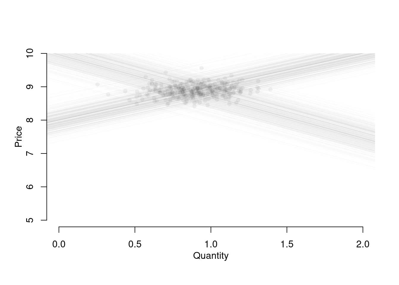
##
## Call:
## lm(formula = Q ~ T * cost, data = dat2)
##
## Residuals:
##      Min       1Q   Median       3Q      Max
## -0.60286 -0.11877  0.00207  0.12656  0.42259
##
## Coefficients:
##               Estimate Std. Error t value Pr(>|t|)
## (Intercept)  8.571e-01  1.999e-02  42.878   <2e-16 ***
## T            2.041e-04  1.151e-04   1.773   0.0767 .
## cost2        6.442e-01  5.647e-02  11.408   <2e-16 ***
## T:cost2     -6.134e-05  1.628e-04  -0.377   0.7065
## ---
## Signif. codes:  0 '***' 0.001 '**' 0.01 '*' 0.05 '.' 0.1 ' ' 1
##
## Residual standard error: 0.1727 on 596 degrees of freedom
## Multiple R-squared:  0.7953, Adjusted R-squared:  0.7943
## F-statistic: 771.9 on 3 and 596 DF,  p-value: < 2.2e-16
Remember that this is effect is local: different magnitudes of the cost shock or different demand curves generally yeild different estimates.
9.3 Difference in Differences (DID)
The basic idea here is to examine how a variable changes in response to an exogenous shock, compared to a control group. Again, there is a large “Applied Statistics” literature I direct you to first
- https://mixtape.scunning.com/09-difference_in_differences
- https://theeffectbook.net/ch-DifferenceinDifference.html
- http://www.urfie.net/read/index.html#page/226
EQ3 <- sapply(1:(2*N), function(n){

    ## Market Mechanisms
    demand <- qd_fun(P)
    supply <- qs_fun(P)

    ## Compute EQ (what we observe)
    eq_id <- which.min( abs(demand-supply) )
    eq <- c(P=P[eq_id], Q=demand[eq_id])

    ## Return Equilibrium Observations
    return(eq)
})
dat3 <- data.frame(t(EQ3), cost='1', T=1:ncol(EQ3))


par(mfrow=c(1,2))
plot(P~T, dat2, main='Effect of Cost Shock on Price', pch=17,col=rgb(0,0,1,.25))
points(P~T, dat3, pch=16, col=rgb(1,0,0,.25))

plot(Q~T, dat2, main='Effect of Cost Shock on Quantity', pch=17,col=rgb(0,0,1,.25))
points(Q~T, dat3, pch=16, col=rgb(1,0,0,.25))
##
## Call:
## lm(formula = P ~ T * cost, data = dat)
##
## Residuals:
##      Min       1Q   Median       3Q      Max
## -0.57978 -0.12392  0.00113  0.12248  0.55214
##
## Coefficients:
##               Estimate Std. Error t value Pr(>|t|)
## (Intercept)  8.900e+00  1.141e-02 780.171   <2e-16 ***
## T           -1.193e-05  3.798e-05  -0.314    0.754
## cost2       -8.415e-01  5.889e-02 -14.289   <2e-16 ***
## T:cost2     -3.577e-06  1.315e-04  -0.027    0.978
## ---
## Signif. codes:  0 '***' 0.001 '**' 0.01 '*' 0.05 '.' 0.1 ' ' 1
##
## Residual standard error: 0.1889 on 1196 degrees of freedom
## Multiple R-squared:  0.7903, Adjusted R-squared:  0.7898
## F-statistic: 1502 on 3 and 1196 DF, p-value: < 2.2e-16##
## Call:
## lm(formula = Q ~ T * cost, data = dat)
##
## Residuals:
## Min 1Q Median 3Q Max
## -0.60286 -0.12032 0.00679 0.13024 0.54253
##
## Coefficients:
## Estimate Std. Error t value Pr(>|t|)
## (Intercept) 8.702e-01 1.071e-02 81.268 <2e-16 ***
## T 8.131e-05 3.564e-05 2.281 0.0227 *
## cost2 6.312e-01 5.528e-02 11.419 <2e-16 ***
## T:cost2 6.149e-05 1.235e-04 0.498 0.6186
## ---
## Signif. codes: 0 '***' 0.001 '**' 0.01 '*' 0.05 '.' 0.1 ' ' 1
##
## Residual standard error: 0.1773 on 1196 degrees of freedom
## Multiple R-squared: 0.7321, Adjusted R-squared: 0.7314
## F-statistic: 1090 on 3 and 1196 DF, p-value: < 2.2e-16Again, the effects are local.