4 Statistics

---

We often summarize distributions with statistics: functions of data. The most basic way to do this is with summary, whose values can all be calculated individually. (E.g., the “mean” computes the [sum of all values] divided by [number of values].) There are many other statistics.

Code

summary( runif(1000))
##      Min.   1st Qu.    Median      Mean   3rd Qu.      Max. 
## 6.534e-05 2.434e-01 5.054e-01 5.040e-01 7.685e-01 9.995e-01
summary( rnorm(1000) )
##     Min.  1st Qu.   Median     Mean  3rd Qu.     Max. 
## -2.84855 -0.65619 -0.05057 -0.02011  0.64258  3.42109

4.1 Mean and Variance

The most basic statistics summarize the center of a distribution and how far apart the values are spread.

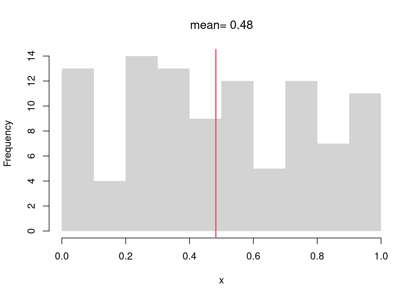
Mean.

Perhaps the most common statistic is the mean; \[\overline{X}=\frac{\sum_{i=1}^{N}X_{i}}{N},\] where \(X_{i}\) denotes the value of the \(i\)th observation.

Code

# compute the mean of a random sample
x <- runif(100)
hist(x, border=NA, main=NA)
m <- mean(x)  #sum(x)/length(x)
abline(v=m, col=2, lwd=2)
title(paste0('mean= ', round(m,2)), font.main=1)

Code

# is m close to it's true value (1-0)/2=.5?

Variance.

Perhaps the second most common statistic is the variance: the average squared deviation from the mean \[V_{X} =\frac{\sum_{i=1}^{N} [X_{i} - \overline{X}]^2}{N}.\] The standard deviation is simply \(s_{X} = \sqrt{V_{X}}\).

Code

s <- sd(x) # sqrt(var(x))
hist(x, border=NA, main=NA, freq=F)
s_lh <- c(m - s,  m + s)
abline(v=s_lh, col=4)
text(s_lh, -.02,
    c( expression(bar(X)-s[X]), expression(bar(X)+s[X])),
    col=4, adj=0)
title(paste0('sd= ', round(s,2)), font.main=1)

Note that a “corrected version” is used by R and many statisticians: \(V_{X} =\frac{\sum_{i=1}^{N} [X_{i} - \overline{X}]^2}{N-1}\).

Code

var(x)
## [1] 0.08561227
mean( (x - mean(x))^2 )
## [1] 0.08475614

Together, these statistics summarize the central tendency and dispersion of a distribution. In some special cases, such as with the normal distribution, they completely describe the distribution. Other distributions are easier to describe with other statistics.

4.2 Other Center/Spread Statistics

Absolute Deviations.

We can use the Median as a “robust alternative” to means. Recall that the \(q\)th quantile is the value where \(q\) percent of the data are below and (\(1-q\)) percent are above. The median (\(q=.5\)) is the point where half of the data is lower values and the other half is higher.

We can also use the Interquartile Range or Median Absolute Deviation as an alternative to variance. The first and third quartiles (\(q=.25\) and \(q=.75\)) together measure is the middle 50 percent of the data. The size of that range (interquartile range: the difference between the quartiles) represents “spread” or “dispersion” of the data. The median absolute deviation also measures spread \[ \tilde{X} = Med(X_{i}) \\ MAD_{X} = Med\left( | X_{i} - \tilde{X} | \right). \]

Code

x <- rgeom(50, .4)
x
##  [1]  2  0  5  0  2  0  0  2  4  3  3  0  0  1  0  3  4  1  2  0  0  6  1  0  1
## [26]  0  1  0  0  0  0  0  3  0  0 11  1  7  2  1  0  8  4  0  2  5  2  0  0  0

plot(table(x))

Code

#mean(x)
median(x)
## [1] 1

#sd(x)
#IQR(x) # diff( quantile(x, probs=c(.25,.75)))
mad(x, constant=1) # median( abs(x - median(x)) )
## [1] 1

Note that there other absolute deviations:

Code

mean( abs(x - mean(x)) )
mean( abs(x - median(x)) )
median( abs(x - mean(x)) )

Mode and Share Concentration.

Sometimes, none of the above work well. With categorical data, for example, distributions are easier to describe with other statistics. The mode is the most common observation: the value with the highest observed frequency. We can also measure the spread/dispersion of the frequencies, or compare the highest frequency to the average frequency to measure concentration at the mode.

Code

# Draw 3 Random Letters
K <- length(LETTERS)
x_id <- rmultinom(3, 1, prob=rep(1/K,K))
x_id
##       [,1] [,2] [,3]
##  [1,]    0    0    0
##  [2,]    0    0    0
##  [3,]    0    0    0
##  [4,]    0    0    0
##  [5,]    0    0    0
##  [6,]    0    0    0
##  [7,]    0    0    0
##  [8,]    0    0    0
##  [9,]    0    0    1
## [10,]    0    0    0
## [11,]    0    0    0
## [12,]    0    0    0
## [13,]    0    0    0
## [14,]    0    0    0
## [15,]    0    0    0
## [16,]    0    0    0
## [17,]    0    0    0
## [18,]    0    0    0
## [19,]    0    0    0
## [20,]    0    1    0
## [21,]    0    0    0
## [22,]    0    0    0
## [23,]    0    0    0
## [24,]    0    0    0
## [25,]    0    0    0
## [26,]    1    0    0

# Draw Random Letters 100 Times
x_id <- rowSums(rmultinom(100, 1, prob=rep(1/K,K)))
x <- lapply(1:K, function(k){
    rep(LETTERS[k], x_id[k])
})
x <- factor(unlist(x), levels=LETTERS)

plot(x)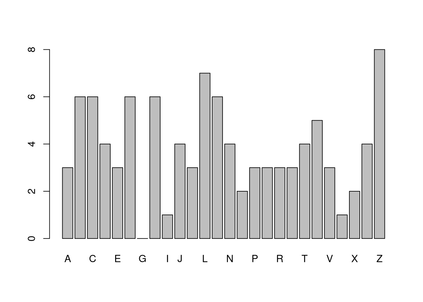

Code

tx <- table(x)
# mode(s)
names(tx)[tx==max(tx)]
## [1] "Z"

# freq. spread
sx <- tx/sum(tx)
sd(sx) # mad(sx)
## [1] 0.01953301

# freq. concentration 
max(tx)/mean(tx)
## [1] 2.08

4.3 Shape Statistics

Central tendency and dispersion are often insufficient to describe a distribution. To further describe shape, we can compute the “standard moments” skew and kurtosis, as well as other statistics.

Skewness.

This captures how symmetric the distribution is. \[Skew_{X} =\frac{\sum_{i=1}^{N} [X_{i} - \overline{X}]^3 / N}{ [s_{X}]^3 }\]

Code

x <- rweibull(1000, shape=1)
hist(x, border=NA, main=NA, freq=F, breaks=20)

Code

skewness <-  function(x) {
 x_bar <- mean(x)
 m3 <- mean((x - x_bar)^3)
 skew <- m3/(sd(x)^3)
 return(skew)
}

skewness( rweibull(1000, shape=1))
## [1] 2.271089
skewness( rweibull(1000, shape=10) )
## [1] -0.5094236

Kurtosis.

This captures how many “outliers” there are. \[Kurt_{X} =\frac{\sum_{i=1}^{N} [X_{i} - \overline{X}]^4 / N}{ [s_{X}]^4 }.\]

Code

x <- rweibull(1000, shape=1)
boxplot(x, main=NA)

Code

kurtosis <- function(x) {  
 x_bar <- mean(x)
 m4 <- mean((x - x_bar)^4) 
 kurt <- m4/(sd(x)^4) - 3  
 return(kurt)
}

kurtosis( rweibull(1000, shape=1))
## [1] 5.471682
kurtosis( rweibull(1000, shape=10) )
## [1] 0.5462298

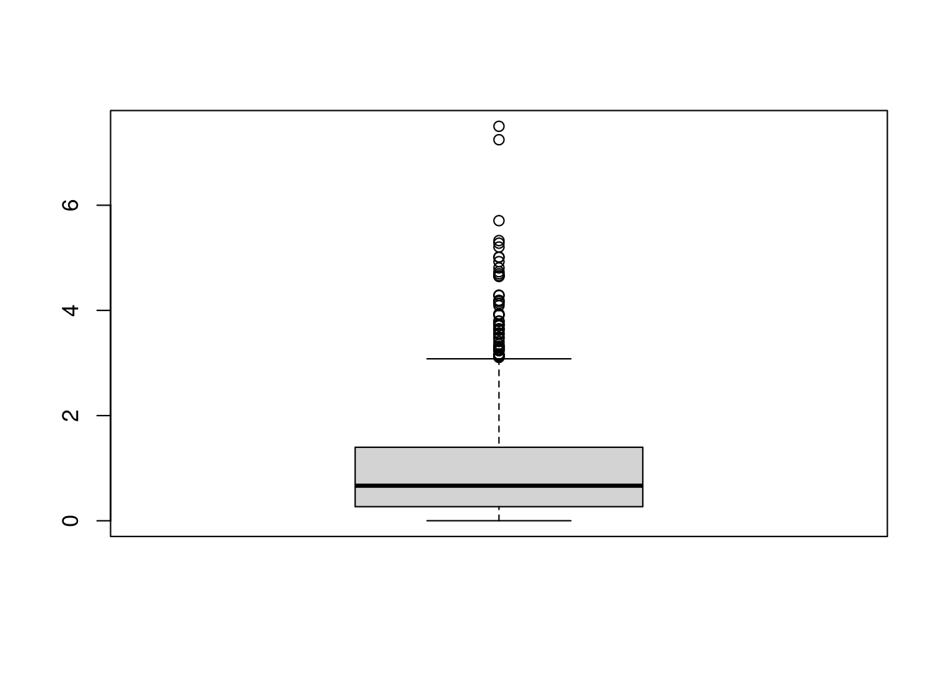
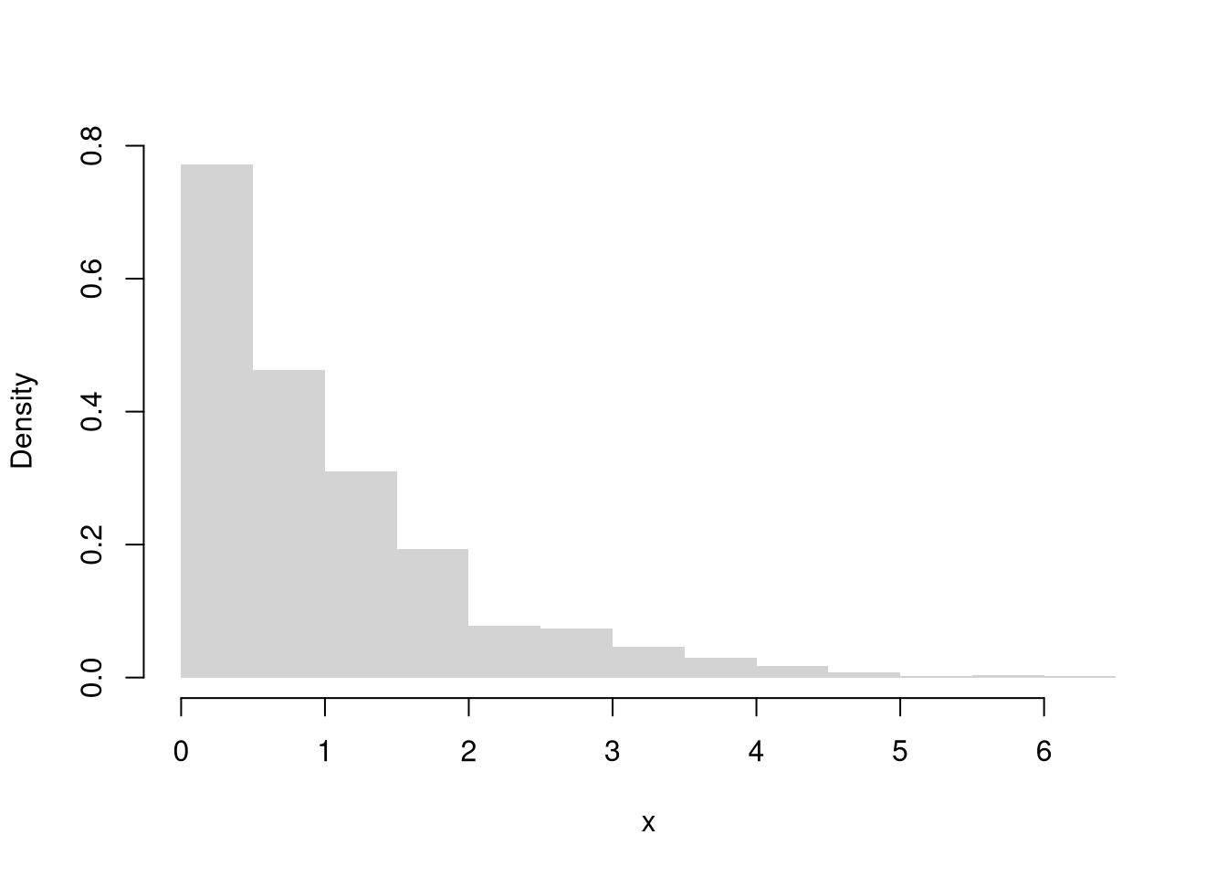
Clusters/Gaps.

You can also describe distributions in terms of how clustered the values are. Remember: a picture is worth a thousand words.

Code

# Number of Modes
x <- rbeta(1000, .6, .6)
hist(x, border=NA, main=NA, freq=F, breaks=20)

Code

# Random Number Generator 
r_ugly1 <- function(n, theta1=c(-8,-1), theta2=c(-2,2), rho=.25){
    omega   <- rbinom(n, size=1, rho)
    epsilon <- omega * runif(n, theta1[1], theta2[1]) +
        (1-omega) * rnorm(n, theta1[2], theta2[2])
    return(epsilon)
}
# Large Sample
par(mfrow=c(1,1))
X <- seq(-12,6,by=.001)
rx <- r_ugly1(1000000)
hist(rx, breaks=1000,  freq=F, border=NA,
    xlab="x", main='')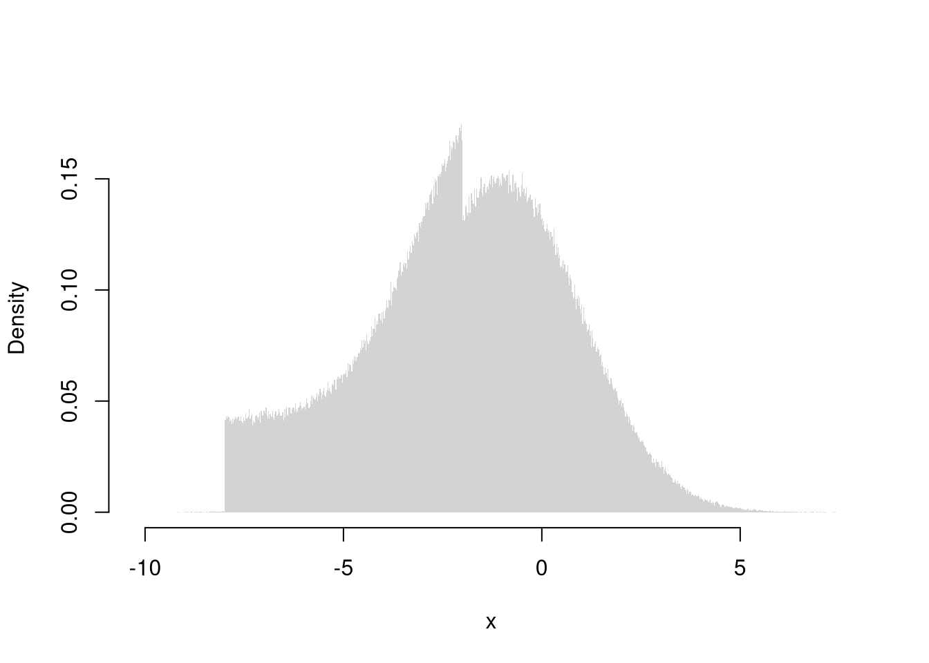

Code

# Show True Density
d_ugly1 <- function(x, theta1=c(-8,-1), theta2=c(-2,2), rho=.25){
    rho     * dunif(x, theta1[1], theta2[1]) +
    (1-rho) * dnorm(x, theta1[2], theta2[2]) }
dx <- d_ugly1(X)
lines(X, dx, col=1)

4.4 Associations

There are several ways to quantitatively describe the relationship between two variables, \(Y\) and \(X\). The major differences surround whether the variables are cardinal, ordinal, or categorical.

Correlation.

Pearson (Linear) Correlation. Suppose \(X\) and \(Y\) are both cardinal data. As such, you can compute the most famous measure of association, the covariance: \[ C_{XY} = \sum_{i} [X_i - \overline{X}] [Y_i - \overline{Y}] / N \]

Code

# Bivariate Data from USArrests
xy <- USArrests[,c('Murder','UrbanPop')]
#plot(xy, pch=16, col=grey(0,.25))
cov(xy)
##             Murder   UrbanPop
## Murder   18.970465   4.386204
## UrbanPop  4.386204 209.518776

Note that \(C_{XX}=V_{X}\). For ease of interpretation, we rescale this statistic to always lay between \(-1\) and \(1\) \[ r_{XY} = \frac{ C_{XY} }{ \sqrt{V_X} \sqrt{V_Y}} \]

Code

cor(xy)[2]
## [1] 0.06957262

Falk Codeviance. The Codeviance is a robust alternative to Covariance. Instead of relying on means (which can be sensitive to outliers), it uses medians (\(\tilde{X}\)) to capture the central tendency.³ We can also scale the Codeviance by the median absolute deviation to compute the median correlation. \[ \text{CoDev}(X,Y) = \text{Med}\left\{ |X_i - \tilde{X}| |Y_i - \tilde{Y}| \right\} \\ \tilde{r}_{XY} = \frac{ \text{CoDev}(X,Y) }{ \text{MAD}(X) \text{MAD}(Y) }. \]

Code

cor_m <- function(xy) {
  # Compute medians for each column
  med <- apply(xy, 2, median)
  # Subtract the medians from each column
  xm <- sweep(xy, 2, med, "-")
  # Compute CoDev
  CoDev <- median(xm[, 1] * xm[, 2])
  # Compute the medians of absolute deviation
  MadProd <- prod( apply(abs(xm), 2, median) )
  # Return the robust correlation measure
  return( CoDev / MadProd)
}
cor_m(xy)
## [1] 0.005707763

Kendall’s Tau.

Suppose \(X\) and \(Y\) are both ordered variables. Kendall’s Tau measures the strength and direction of association by counting the number of concordant pairs (where the ranks agree) versus discordant pairs (where the ranks disagree). A value of \(\tau = 1\) implies perfect agreement in rankings, \(\tau = -1\) indicates perfect disagreement, and \(\tau = 0\) suggests no association in the ordering. \[ \tau = \frac{2}{n(n-1)} \sum_{i} \sum_{j > i} \text{sgn} \Bigl( (X_i - X_j)(Y_i - Y_j) \Bigr), \] where the sign function is: \[ \text{sgn}(z) = \begin{cases} +1 & \text{if } z > 0\\ 0 & \text{if } z = 0 \\ -1 & \text{if} z < 0 \end{cases}. \]

Code

xy <- USArrests[,c('Murder','UrbanPop')]
xy[,1] <- rank(xy[,1] )
xy[,2] <- rank(xy[,2] )
# plot(xy, pch=16, col=grey(0,.25))
tau <- cor(xy[, 1], xy[, 2], method = "kendall")
round(tau, 3)
## [1] 0.074

Cramer’s V.

Suppose \(X\) and \(Y\) are both categorical variables; the value of \(X\) is one of \(1...r\) categories and the value of \(Y\) is one of \(1...k\) categories. Cramer’s V quantifies the strength of association by adjusting a “chi-squared” statistic to provide a measure that ranges from 0 to 1; 0 indicates no association while a value closer to 1 signifies a strong association.

First, consider a contingency table for \(X\) and \(Y\) with \(r\) rows and \(k\) columns. The chi-square statistic is then defined as:

\[ \chi^2 = \sum_{i=1}^{r} \sum_{j=1}^{k} \frac{(O_{ij} - E_{ij})^2}{E_{ij}}. \]

where

• \(O_{ij}\) denote the observed frequency in cell \((i, j)\),
• \(E_{ij} = \frac{R_i \cdot C_j}{n}\) is the expected frequency for each cell if \(X\) and \(Y\) are independent
• \(R_i\) denote the total frequency for row \(i\) (i.e., \(R_i = \sum_{j=1}^{k} O_{ij}\)),
• \(C_j\) denote the total frequency for column \(j\) (i.e., \(C_j = \sum_{i=1}^{r} O_{ij}\)),
• \(n\) be the grand total of observations, so that \(n = \sum_{i=1}^{r} \sum_{j=1}^{k} O_{ij}\).

Second, normalize the chi-square statistic with the sample size and the degrees of freedom to compute Cramer’s V.

\[ V = \sqrt{\frac{\chi^2 / n}{\min(k - 1, \, r - 1)}}, \]

where:

• \(n\) is the total sample size,
• \(k\) is the number of categories for one variable,
• \(r\) is the number of categories for the other variable.

Code

xy <- USArrests[,c('Murder','UrbanPop')]
xy[,1] <- cut(xy[,1],3)
xy[,2] <- cut(xy[,2],4)
table(xy)
##               UrbanPop
## Murder         (31.9,46.8] (46.8,61.5] (61.5,76.2] (76.2,91.1]
##   (0.783,6.33]           4           5           8           5
##   (6.33,11.9]            0           4           7           6
##   (11.9,17.4]            2           4           2           3

cor_v <- function(xy){
    # Create a contingency table from the categorical variables
    tbl <- table(xy)
    # Compute the chi-square statistic (without Yates' continuity correction)
    chi2 <- chisq.test(tbl, correct=FALSE)$statistic
    # Total sample size
    n <- sum(tbl)
    # Compute the minimum degrees of freedom (min(rows-1, columns-1))
    df_min <- min(nrow(tbl) - 1, ncol(tbl) - 1)
    # Calculate Cramer's V
    V <- sqrt((chi2 / n) / df_min)
    return(V)
}
cor_v(xy)
## X-squared 
## 0.2307071

# DescTools::CramerV( table(xy) )

4.5 Beyond Basics

Use expansion “packages” for less common procedures and more functionality

CRAN.

Most packages can be found on CRAN and can be easily installed

Code

# commonly used packages
install.packages("stargazer")
install.packages("data.table")
install.packages("plotly")
# other statistical packages
install.packages("extraDistr")
install.packages("twosamples")
# install.packages("purrr")
# install.packages("reshape2")

The most common tasks also have cheatsheets you can use.

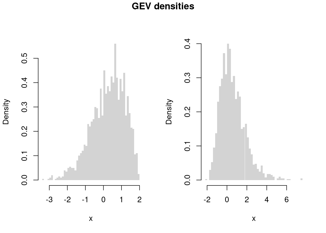
For example, to generate ‘exotic’ probability distributions

Code

library(extraDistr)

par(mfrow=c(1,2))
for(p in c(-.5,0)){
    x <- rgev(2000, mu=0, sigma=1, xi=p)
    hist(x, breaks=50, border=NA, main=NA, freq=F)
}
title('GEV densities', outer=T, line=-1)

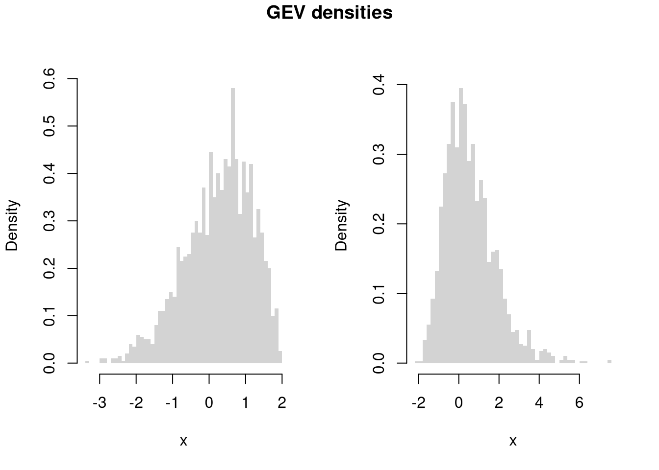
Code

library(extraDistr)

par(mfrow=c(1,3))
for(p in c(-1, 0,2)){
    x <- rtlambda(2000, p)
    hist(x, breaks=100, border=NA, main=NA, freq=F)
}
title('Tukey-Lambda densities', outer=T, line=-1)

Github.

Sometimes you will want to install a package from GitHub. For this, you can use devtools or its light-weight version remotes

Code

install.packages("devtools")
install.packages("remotes")

Note that to install devtools, you also need to have developer tools installed on your computer.

• Windows: Rtools
• Mac: Xcode

To color terminal output on Linux systems, you can use the colorout package

Code

library(remotes)
# Install https://github.com/jalvesaq/colorout
# to .libPaths()[1]
install_github('jalvesaq/colorout')
library(colorout)

Base.

While additional packages can make your code faster, they also create dependancies that can lead to problems. So learn base R well before becoming dependant on other packages

• https://bitsofanalytics.org/posts/base-vs-tidy/
• https://jtr13.github.io/cc21fall2/comparison-among-base-r-tidyverse-and-datatable.html

4.6 Further Reading

Many random variables are related to each other

• https://en.wikipedia.org/wiki/Relationships_among_probability_distributions
• https://www.math.wm.edu/~leemis/chart/UDR/UDR.html
• https://qiangbo-workspace.oss-cn-shanghai.aliyuncs.com/2018-11-11-common-probability-distributions/distab.pdf

Note that numbers randomly generated on your computer cannot be truly random, they are “Pseudorandom”.

---

3. See also Theil-Sen Estimator, which may be seen as a precursor.↩︎