7 Simple OLS
Model and objective \[ y_i=\alpha+\beta x_i+\epsilon_{i} \\ \epsilon_{i} = y_i - [\alpha+\beta x_i]\\ min_{\beta} \sum_{i=1}^{n} (\epsilon_{i})^2 \]
Point Estimates \[ \hat{\alpha}=\bar{y}-\hat{\beta}\bar{x} = \widehat{\mathbb{E}}[Y] - \hat{\beta} \widehat{\mathbb{E}}[X] \\ \hat{\beta}=\frac{\sum_{i}^{}(x_i-\bar{x})(y_i-\bar{y})}{\sum_{i}^{}(x_i-\bar{x})^2} = \frac{\widehat{Cov}[X,Y]}{\widehat{\mathbb{V}}[X]}\\ \hat{y}_i=\hat{\alpha}+\hat{\beta}x_i\\ \hat{\epsilon}_i=y_i-\hat{y}_i\\ \]
Before fitting the model to your data, explore your data (as in Part I)
## Inspect Dataset
xy <- USArrests[,c('Murder','UrbanPop')]
colnames(xy) <- c('y','x')
## head(xy)
## Plot Data
plot(y~x, xy, col=grey(.5,.5), pch=16)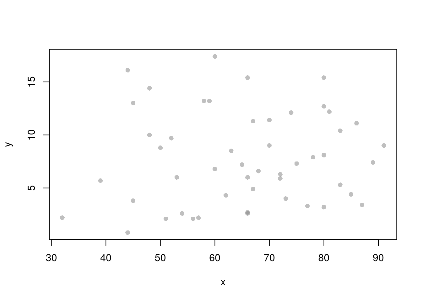
##
## Call:
## lm(formula = y ~ x, data = xy)
##
## Coefficients:
## (Intercept)            x
##     6.41594      0.02093
## (Intercept) x
## 6.41594246 0.02093466To measure the ‘’Goodness of fit’’, we analyze sums of squared errors (Total, Explained, and Residual) as \[ \underbrace{\sum_{i}(y_i-\bar{y})^2}_\text{TSS}=\underbrace{\sum_{i}(\hat{y}_i-\bar{y})^2}_\text{ESS}+\underbrace{\sum_{i}\hat{\epsilon_{i}}^2}_\text{RSS}\\ R^2 = \frac{ESS}{TSS}=1-\frac{RSS}{TSS} \] Note that \(R^2\) is also called the coefficient of determination.
## Manually Compute Goodness of Fit
Ehat <- resid(reg)
RSS  <- sum(Ehat^2)
Y <- xy$y
TSS  <- sum((Y-mean(Y))^2)
R2 <- 1 - RSS/TSS
R2
## [1] 0.00484035## [1] 0.004840357.1 Variability Estimates
A regression coefficient is a statistic. And, just like all statistics, we can calculate
- standard deviation: variability within a single sample.
- standard error: variability across different samples.
- confidence interval: range your statistic varies across different samples.
- null distribution: the sampling distribution of the statistic under the null hypothesis (assuming your null hypothesis was true).
- p-value the probability you would see something as extreme as your statistic when sampling from the null distribution.
To calculate these variability statistics, we will estimate variabilty using data-driven methods.1
We first consider the simplest, the jackknife. In this procedure, we loop through each row of the dataset. And, in each iteration of the loop, we drop that observation from the dataset and reestimate the statistic of interest. We then calculate the standard deviation of the statistic across all ``resamples’’.
## Example 1 Continued

## Jackknife Standard Errors for Beta
jack_regs <- lapply(1:nrow(xy), function(i){
    xy_i <- xy[-i,]
    reg_i <- lm(y~x, dat=xy_i)
})
jack_coefs <- sapply(jack_regs, coef)['x',]
jack_mean <- mean(jack_coefs)
jack_se <- sd(jack_coefs)

## Jackknife Confidence Intervals
jack_ci_percentile <- quantile(jack_coefs, probs=c(.025,.975))
hist(jack_coefs, breaks=25,
    main=paste0('SE est. = ', round(jack_se,4)),
    xlab=expression(beta[-i]))
abline(v=jack_mean, col="red", lwd=2)
abline(v=jack_ci_percentile, col="red", lty=2)
## Plot Full-Sample Estimate
## abline(v=coef(reg)['x'], lty=1, col='blue', lwd=2)

## Plot Normal Approximation
## jack_ci_normal <- jack_mean+c(-1.96, +1.96)*jack_se
## abline(v=jack_ci_normal, col="red", lty=3)
There are several other resampling techniques. We consider the other main one, the bootstrap, which resamples with replacement for an arbitrary number of iterations. When bootstrapping a dataset with \(n\) observations, you randomly resample all \(n\) rows in your data set \(B\) times.
| Sample Size per Iteration | Number of Iterations | Resample | |
|---|---|---|---|
| Bootstrap | \(n\) | \(B\) | With Replacement |
| Jackknife | \(n-1\) | \(n\) | Without Replacement |
## Bootstrap Standard Errors for Beta
boots <- 1:399
boot_regs <- lapply(boots, function(b){
    b_id <- sample( nrow(xy), replace=T)
    xy_b <- xy[b_id,]
    reg_b <- lm(y~x, dat=xy_b)
})
boot_coefs <- sapply(boot_regs, coef)['x',]
boot_mean <- mean(boot_coefs)
boot_se <- sd(boot_coefs)

## Bootstrap Confidence Intervals
boot_ci_percentile <- quantile(boot_coefs, probs=c(.025,.975))
hist(boot_coefs, breaks=25,
    main=paste0('SE est. = ', round(boot_se,4)),
    xlab=expression(beta[b]))
abline(v=boot_mean, col="red", lwd=2)
abline(v=boot_ci_percentile, col="red", lty=2)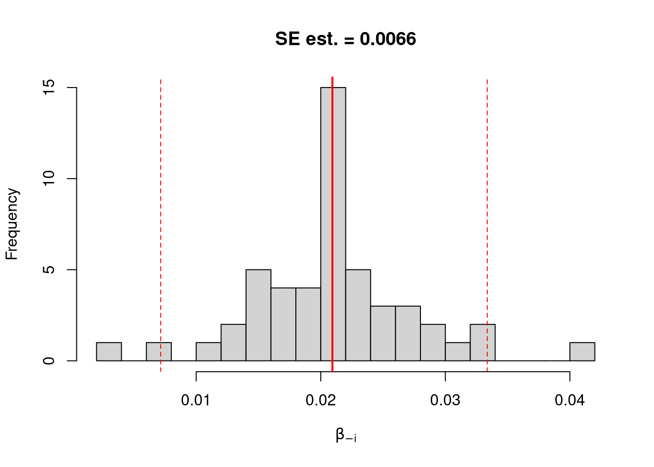
## Normal Approximation
## boot_ci_normal <- boot_mean+c(-1.96, +1.96)*boot

## Parametric CI
## x <- data.frame(x=quantile(xy$x,probs=seq(0,1,by=.1)))
## ci <- predict(reg, interval='confidence', newdata=data.frame(x))
## polygon( c(x, rev(x)), c(ci[,'lwr'], rev(ci[,'upr'])), col=grey(0,.2), border=0)
We can also bootstrap other statistics, such as a t-statistic or \(R^2\). We do such things to test a null hypothesis, which is often ``no relationship’’. We are rarely interested in computing standard errrors and conducting hypothesis tests for two variables. However, we work through the ideas in the two-variable case to better understand the multi-variable case.
7.2 Hypothesis Tests
There are two main ways to conduct a hypothesis test.
Invert a CI One main way to conduct hypothesis tests is to examine whether a confidence interval contains a hypothesized value. Often, this is \(0\).
## Example 1 Continued Yet Again

## Bootstrap Distribution
boot_ci_percentile <- quantile(boot_coefs, probs=c(.025,.975))
hist(boot_coefs, breaks=25,
    main=paste0('SE est. = ', round(boot_se,4)),
    xlab=expression(beta[b]),
    xlim=range(c(0, boot_coefs)) )
abline(v=boot_ci_percentile, lty=2, col="red")
abline(v=0, col="red", lwd=2)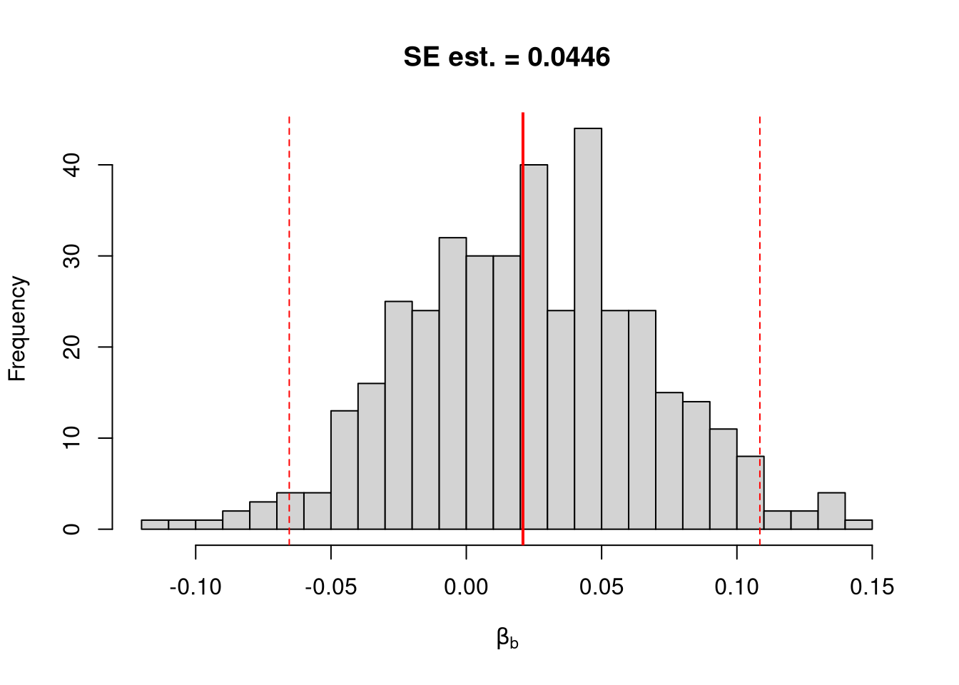
Impose the Null We can also compute a null distribution using data-driven methods that assume much less about the data generating process. We focus on the simplest, the bootstrap, where loop through a large number of simulations. In each iteration of the loop, we drop impose the null hypothesis and reestimate the statistic of interest. We then calculate the standard deviation of the statistic across all ``resamples’’.
## Example 1 Continued Again

## Null Distribution for Beta
boots <- 1:399
boot_regs0 <- lapply(boots, function(b){
    xy_b <- xy
    xy_b$y <- sample( xy_b$y, replace=T)
    reg_b <- lm(y~x, dat=xy_b)
})
boot_coefs0 <- sapply(boot_regs0, coef)['x',]

## Null Bootstrap Distribution
boot_ci_percentile0 <- quantile(boot_coefs0, probs=c(.025,.975))
hist(boot_coefs0, breaks=25, main='',
    xlab=expression(beta[b]),
    xlim=range(c(boot_coefs0, coef(reg)['x'])))
abline(v=boot_ci_percentile0, col="red", lty=2)
abline(v=coef(reg)['x'], col="red", lwd=2)
Regardless of how we calculate standard errors, we can use them to conduct a t-test. We also compute the distribution of t-values under the null hypothesis, and compare how extreme the oberved value is. \[ \hat{t} = \frac{\hat{\beta} - \beta_{0} }{\hat{\sigma}_{\hat{\beta}}} \]
## T Test
B0 <- 0
boot_t  <- (coef(reg)['x']-B0)/boot_se

## Compute Bootstrap T-Values (without refinement)
boot_t_boot0 <- sapply(boot_regs0, function(reg_b){
    beta_b <- coef(reg_b)[['x']]
    t_hat_b <- (beta_b)/boot_se
    return(t_hat_b)
})
hist(boot_t_boot0, breaks=100,
    main='Bootstrapped t values', xlab='t',
    xlim=range(c(boot_t_boot0, boot_t)) )
abline(v=boot_t, lwd=2, col='red')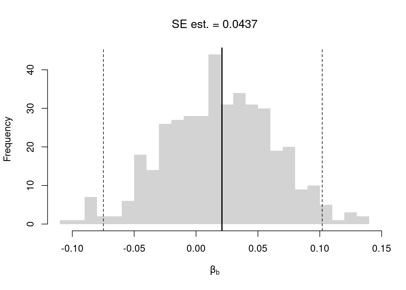
From this, we can calculate a p-value: the probability you would see something as extreme as your statistic under the null (assuming your null hypothesis was true). Note that the \(p\) reported by your computer does not necessarily satisfy this definition. We can always calcuate a p-value from an explicit null distribution.
## One Sided Test for P(t > boot_t | Null)=1- P(t < boot_t | Null)
That_NullDist1 <- ecdf(boot_t_boot0)
Phat1  <- 1-That_NullDist1(boot_t)

## Two Sided Test for P(t > jack_t or  t < -jack_t | Null)
That_NullDist2 <- ecdf(abs(boot_t_boot0))
plot(That_NullDist2, xlim=range(boot_t_boot0, boot_t))
abline(v=quantile(That_NullDist2,probs=.95), lty=3)
abline(v=boot_t, col='red')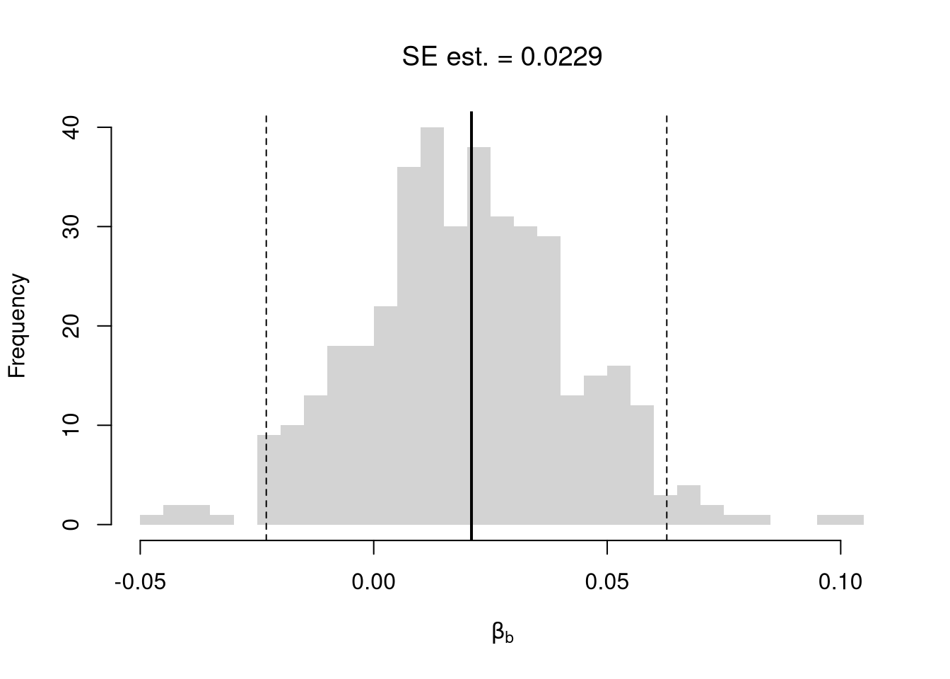
## [1] 0.6240602Under some assumptions, the null distribution is distributed \(t_{n-2}\). (For more on parametric t-testing based on statistical theory, see https://www.econometrics-with-r.org/4-lrwor.html.)
7.3 Prediction Intervals
In addition to confidence intervales, we can also compute a prediction interval which estimates the range of variability across different samples for the outcomes. These intervals also take into account the residuals— the variability of individuals around the mean.
## Bootstrap Prediction Interval
boot_resids <- lapply(boot_regs, function(reg_b){
    e_b <- resid(reg_b)
    x_b <- reg_b$model$x
    res_b <- cbind(e_b, x_b)
})
boot_resids <- as.data.frame(do.call(rbind, boot_resids))
## Homoskedastic
ehat <- quantile(boot_resids$e_b, probs=c(.025, .975))
x <- quantile(xy$x,probs=seq(0,1,by=.1))
boot_pi <- coef(reg)[1] + x*coef(reg)['x']
boot_pi <- cbind(boot_pi + ehat[1], boot_pi + ehat[2])

## Plot Bootstrap PI
plot(y~x, dat=xy, pch=16, main='Prediction Intervals',
ylim=c(-5,20))
polygon( c(x, rev(x)), c(boot_pi[,1], rev(boot_pi[,2])),
    col=grey(0,.2), border=NA)

## Parametric PI (For Comparison)
pi <- predict(reg, interval='prediction', newdata=data.frame(x))
lines( x, pi[,'lwr'], lty=2)
lines( x, pi[,'upr'], lty=2)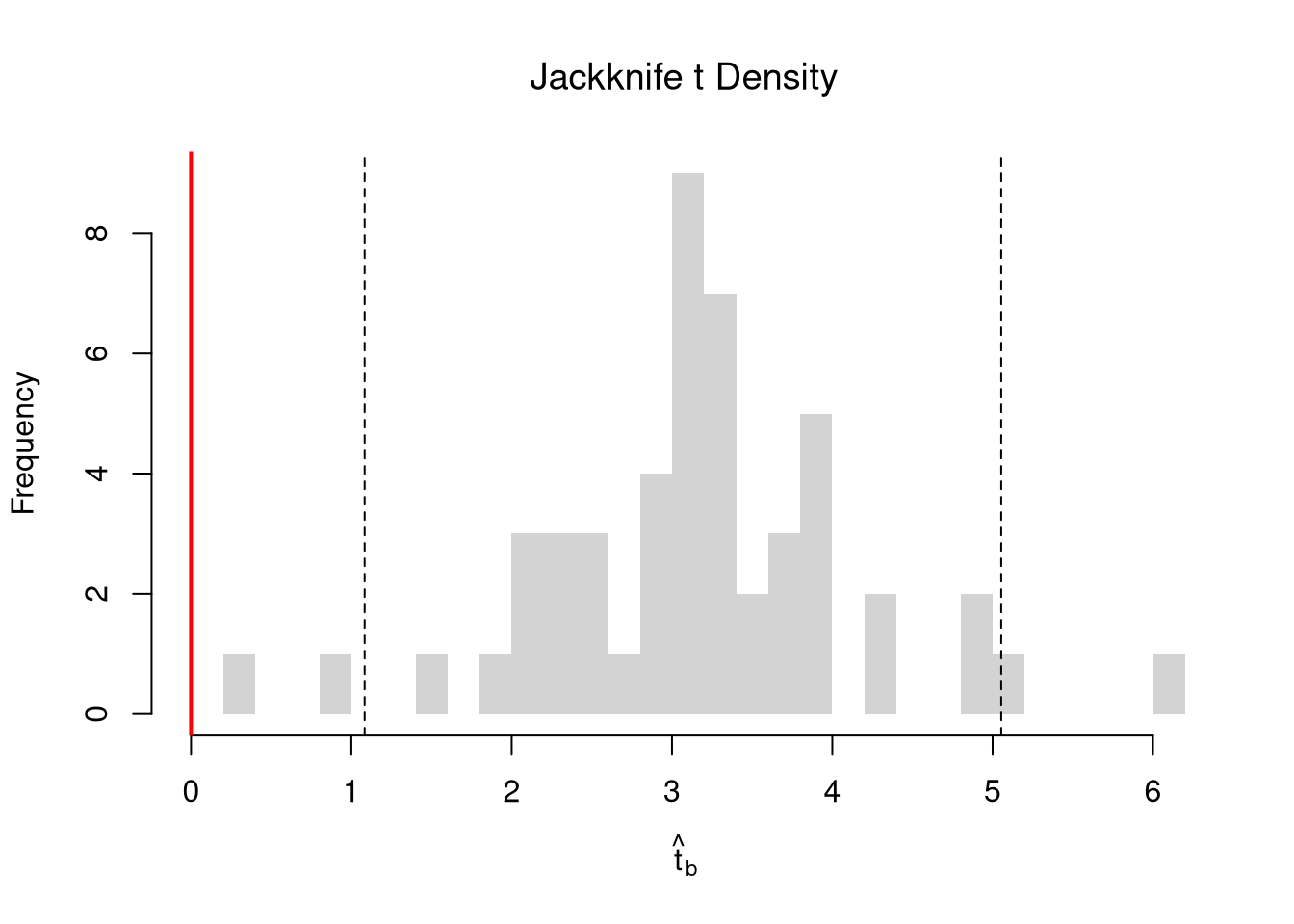
There are many ways to improve upon the prediction intervals you just created. Probably the most basic way is to allow the residuals to be heteroskedastic.
## Estimate Residual Quantiles seperately around X points
boot_resid_list <- split(boot_resids,
    cut(boot_resids$x_b, x) )
boot_resid_est <- lapply(boot_resid_list, function(res_b) {
    if( nrow(res_b)==0){ ## If Empty, Return Nothing
        ehat <- c(NA,NA)
    } else{ ## Estimate Quantiles of Residuals
        ehat <- quantile(res_b$e_b, probs=c(.025, .975))
    }
    return(ehat)
    })
boot_resid_est <- do.call(rbind, boot_resid_est)
## Construct PI at x points
boot_x <- x[-1] - diff(x)/2
boot_pi <- coef(reg)[1] + boot_x*coef(reg)['x']
boot_pi <- cbind(boot_pi + boot_resid_est[,1], boot_pi + boot_resid_est[,2])

plot(y~x, dat=xy, pch=16, main='Heteroskedastic P.I.')
polygon( c(boot_x, rev(boot_x)), c(boot_pi[,1], rev(boot_pi[,2])),
    col=grey(0,.2), border=NA)
rug(boot_x)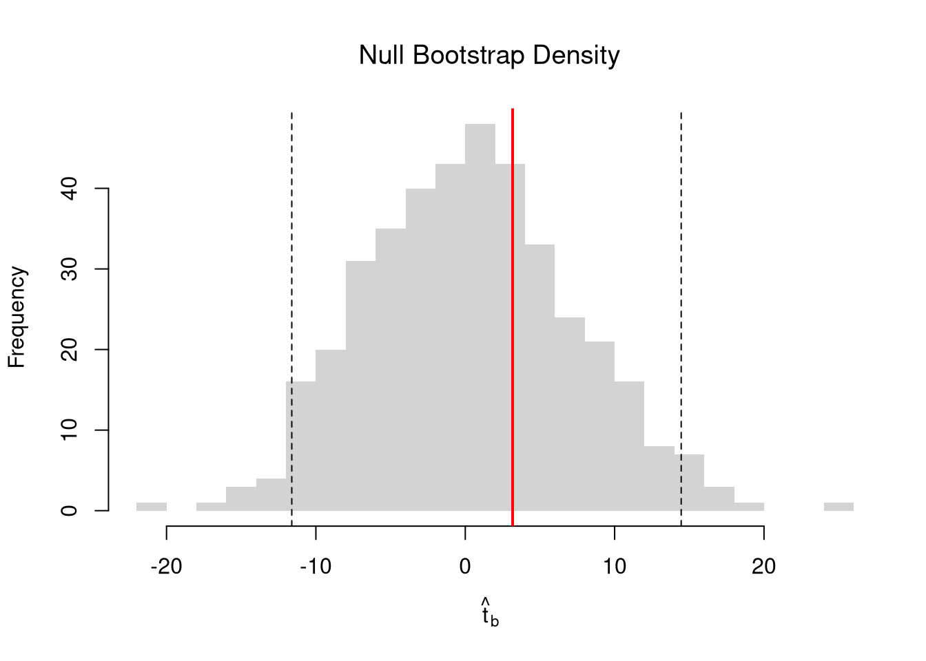
For a nice overview of different types of intervals, see https://www.jstor.org/stable/2685212. For an indepth view, see “Statistical Intervals: A Guide for Practitioners and Researchers” or “Statistical Tolerance Regions: Theory, Applications, and Computation”. See https://robjhyndman.com/hyndsight/intervals/ for constructing intervals for future observations in a time-series context. See Davison and Hinkley, chapters 5 and 6 (also Efron and Tibshirani, or Wehrens et al.)
7.4 Value of More Data
Just as before, there are diminishing returns to larger sample sizes with simple OLS.
B <- 300
Nseq <- seq(3,100, by=1)
SE <- sapply(Nseq, function(n){
    sample_statistics <- sapply(1:B, function(b){
        x <- rnorm(n)
        e <- rnorm(n)
        y <- x*2 + e
        reg <- lm(y~x)
        coef(reg)
        #se <- sqrt(diag(vcov(vcov)))
    })
    sd(sample_statistics)
})

par(mfrow=c(1,2))
plot(Nseq, SE, pch=16, col=grey(0,.5), main='Absolute Gain',
    ylab='standard error', xlab='sample size')
plot(Nseq[-1], abs(diff(SE)), pch=16, col=grey(0,.5), main='Marginal Gain',
    ylab='decrease in standard error', xlab='sample size')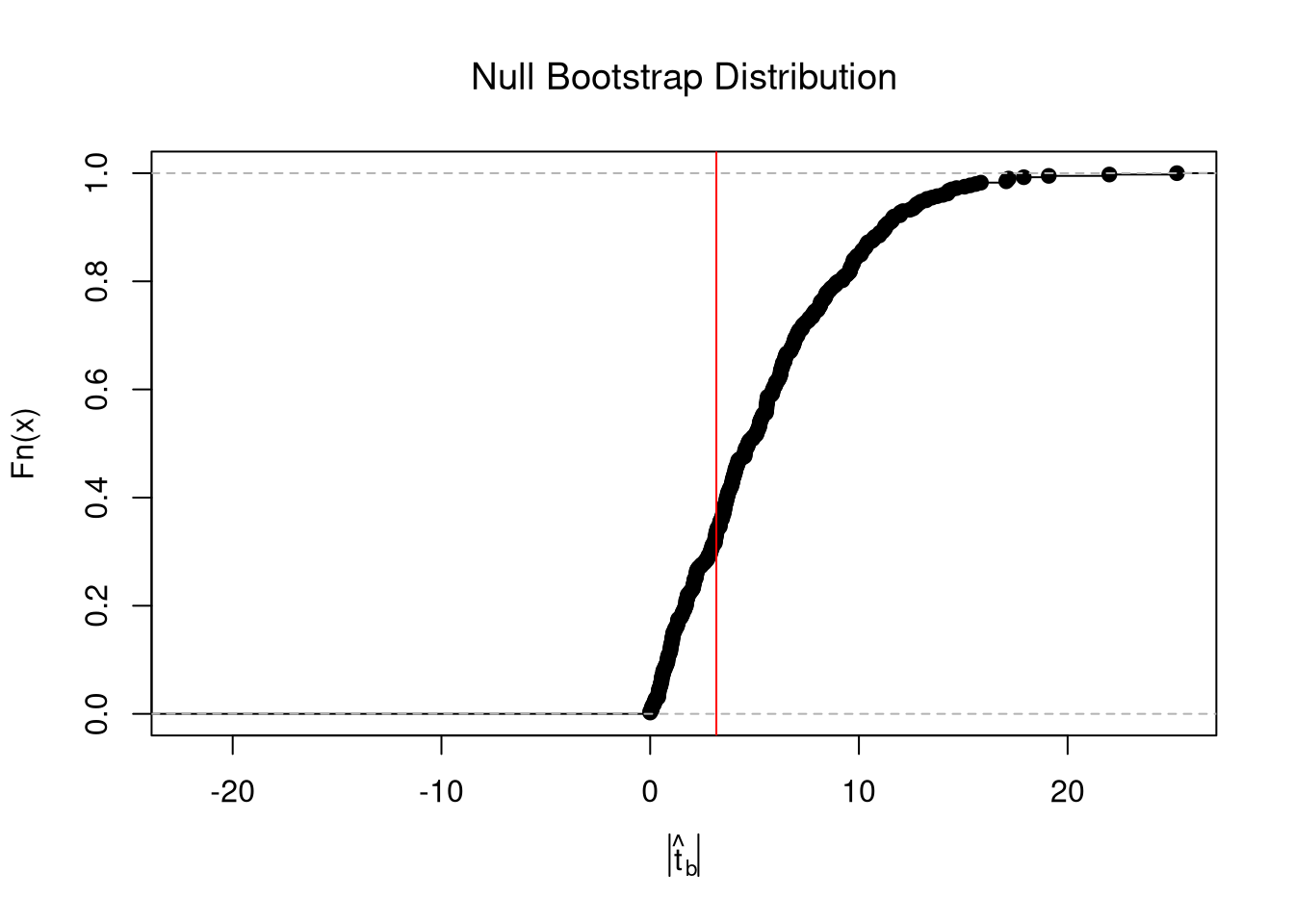
7.5 Locally Linear
Segmented/piecewise regression
## Loading required package: car## Loading required package: carData## Loading required package: lmtest## Loading required package: zoo##
## Attaching package: 'zoo'## The following objects are masked from 'package:base':
##
## as.Date, as.Date.numeric## Loading required package: sandwich## Loading required package: survivaldata(CASchools)
CASchools$score <- (CASchools$read + CASchools$math) / 2
reg <- lm(score ~ income, data = CASchools)
plot( CASchools$income, resid(reg), pch=16, col=grey(0,.5))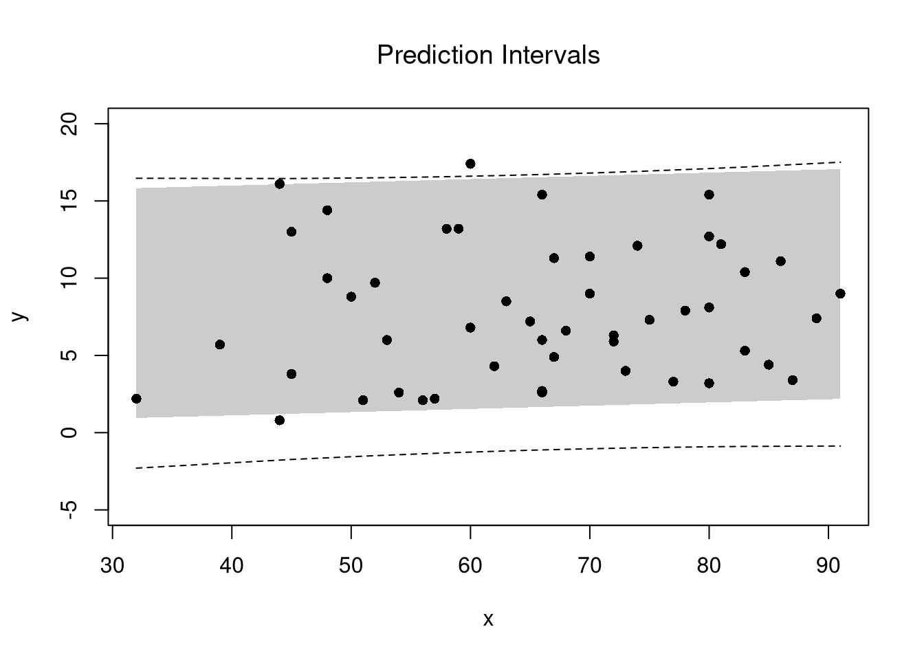
## Add Piecewise Term
CASchools$IncomeCut <- cut(CASchools$income,2)
reg2 <- lm(score ~ income*IncomeCut, data=CASchools)
summary(reg2)
##
## Call:
## lm(formula = score ~ income * IncomeCut, data = CASchools)
##
## Residuals:
## Min 1Q Median 3Q Max
## -44.710 -8.897 0.730 8.210 32.445
##
## Coefficients:
## Estimate Std. Error t value Pr(>|t|)
## (Intercept) 617.4010 2.1013 293.821 < 2e-16 ***
## income 2.4732 0.1426 17.338 < 2e-16 ***
## IncomeCut(30.3,55.4] 59.6336 16.9170 3.525 0.00047 ***
## income:IncomeCut(30.3,55.4] -2.0904 0.4499 -4.646 4.55e-06 ***
## ---
## Signif. codes: 0 '***' 0.001 '**' 0.01 '*' 0.05 '.' 0.1 ' ' 1
##
## Residual standard error: 12.88 on 416 degrees of freedom
## Multiple R-squared: 0.5462, Adjusted R-squared: 0.5429
## F-statistic: 166.9 on 3 and 416 DF, p-value: < 2.2e-16## Analysis of Variance Table
##
## Model 1: score ~ income
## Model 2: score ~ income * IncomeCut
## Res.Df RSS Df Sum of Sq F Pr(>F)
## 1 418 74905
## 2 416 69033 2 5871.7 17.692 4.226e-08 ***
## ---
## Signif. codes: 0 '***' 0.001 '**' 0.01 '*' 0.05 '.' 0.1 ' ' 1## Chow Test for Break
data_splits <- split(CASchools, CASchools$IncomeCut)
resids <- sapply(data_splits, function(dat){
reg <- lm(score ~ income, data=dat)
sum( resid(reg)^2)
})
Ns <- sapply(data_splits, function(dat){ nrow(dat)})
Rt <- (sum(resid(reg)^2) - sum(resids))/sum(resids)
Rb <- (sum(Ns)-2*reg$rank)/reg$rank
Ft <- Rt*Rb
pf(Ft,reg$rank, sum(Ns)-2*reg$rank,lower.tail=F)## [1] 4.225896e-08Multiple Breaks
CASchools$IncomeCut2 <- cut(CASchools$income, seq(0,60,by=20)) ## Finer Bins
reg3 <- lm(score ~ income*IncomeCut2, data=CASchools)
summary(reg3)
##
## Call:
## lm(formula = score ~ income * IncomeCut2, data = CASchools)
##
## Residuals:
## Min 1Q Median 3Q Max
## -42.323 -9.048 0.258 8.279 31.702
##
## Coefficients:
## Estimate Std. Error t value Pr(>|t|)
## (Intercept) 612.0820 2.7523 222.386 < 2e-16 ***
## income 2.9200 0.2073 14.089 < 2e-16 ***
## IncomeCut2(20,40] 23.0794 8.7824 2.628 0.008910 **
## IncomeCut2(40,60] 89.1941 37.6356 2.370 0.018249 *
## income:IncomeCut2(20,40] -1.3601 0.3805 -3.574 0.000393 ***
## income:IncomeCut2(40,60] -3.0429 0.8525 -3.570 0.000400 ***
## ---
## Signif. codes: 0 '***' 0.001 '**' 0.01 '*' 0.05 '.' 0.1 ' ' 1
##
## Residual standard error: 12.78 on 414 degrees of freedom
## Multiple R-squared: 0.5553, Adjusted R-squared: 0.5499
## F-statistic: 103.4 on 5 and 414 DF, p-value: < 2.2e-16## Make Predictions
income <- seq(min(CASchools$income), max(CASchools$income), length.out=1001)
newdata <- data.frame(income,
IncomeCut=cut(income,2),
IncomeCut2=cut(income,seq(0,60,by=20)))
pred1 <- predict(reg, newdata=newdata)
pred2 <- predict(reg2, newdata=newdata)
pred3 <- predict(reg3,newdata=newdata)
## Compare Predictions
plot(score ~ income, pch=16, col=grey(0,.5), dat=CASchools)
lines(income, pred1, lwd=2, col=2)
lines(income, pred2, lwd=2, col=4)
lines(income, pred3, lwd=2, col=3)
legend('topleft',
legend=c('OLS','Peicewise Linear (2)','Peicewise Linear (3)'),
lty=1, col=c(2,4,3), cex=.8)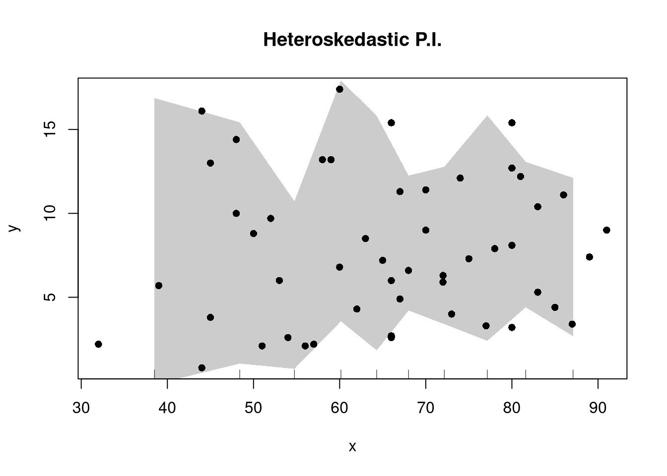
## To Test for Any Break
## strucchange::sctest(score ~ income, data=CASchools, type="Chow", point=.5)
## strucchange::Fstats(score ~ income, data=CASchools)

## To Find Changes
## segmented::segmented(reg)
Smoothing (Linear Regression using subsample around each data point)
plot(score ~ income, pch=16, col=grey(0,.5), dat=CASchools)

## design points
CASchoolsO <- CASchools[order(CASchools$income),]

## Loess (adaptive subsamples)
reg_lo <- loess(score ~ income, data=CASchoolsO,
    span=.8)
lines(CASchoolsO$income, predict(reg_lo),
    col='orange', type='o', pch=8)

## llls (fixed width subsamples)
library(np)
## Nonparametric Kernel Methods for Mixed Datatypes (version 0.60-17)
## [vignette("np_faq",package="np") provides answers to frequently asked questions]
## [vignette("np",package="np") an overview]
## [vignette("entropy_np",package="np") an overview of entropy-based methods]reg_np <- npreg(score ~ income, data=CASchoolsO,
bws=2, bandwidth.compute=F)
lines(CASchoolsO$income, predict(reg_np),
col='purple', type='o', pch=12)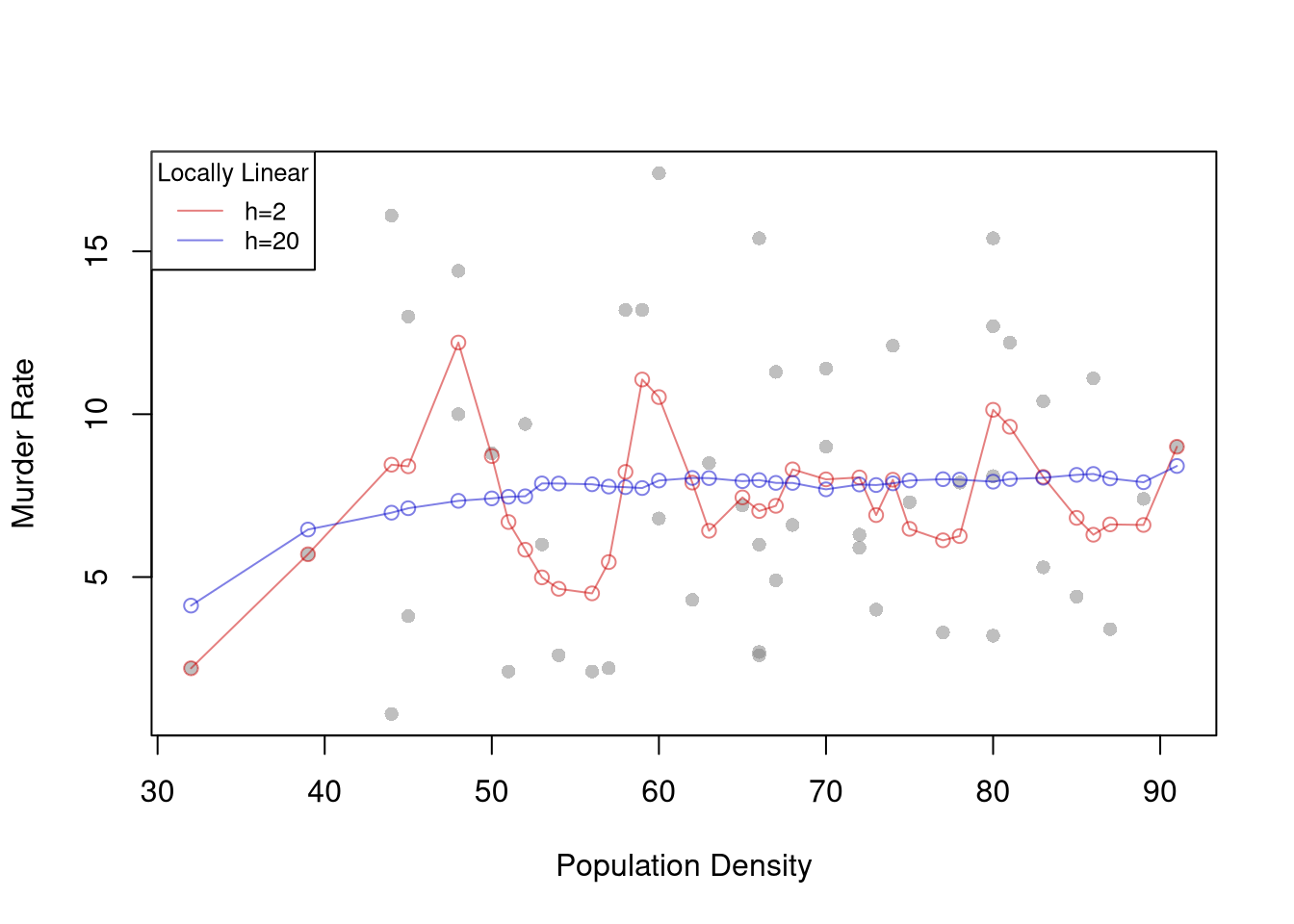
For some technical background, see, e.g., https://www.sagepub.com/sites/default/files/upm-binaries/21122_Chapter_21.pdf. Also note that we can compute classic estimates for variability: denoting the Standard Error of the Regression as \(\hat{\sigma}\), and the Standard Error of the Coefficient Estimates as \(\hat{\sigma}_{\hat{\alpha}}\) and \(\hat{\sigma}_{\hat{\beta}}~~\) (or simply Standard Errors). \[ \hat{\sigma}^2 = \frac{1}{n-2}\sum_{i}\hat{\epsilon_{i}}^2\\ \hat{\sigma}^2_{\hat{\alpha}}=\hat{\sigma}^2\left[\frac{1}{n}+\frac{\bar{x}^2}{\sum_{i}(x_i-\bar{x})^2}\right]\\ \hat{\sigma}^2_{\hat{\beta}}=\frac{\hat{\sigma}^2}{\sum_{i}(x_i-\bar{x})^2}. \] These equations are motivated by particular data generating proceses, which you can read more about this at https://www.econometrics-with-r.org/4-lrwor.html.↩︎