11 Small Scale Projects
11.1 An R Code Chunk
Save the following code as CodeChunk.R
sum_squared <- function(x1, x2) {
    y <- (x1 + x2)^2
    return(y)
}

x <- c(0,1,3,10,6)
sum_squared(x[1], x[3])
sum_squared(x, x[2])
sum_squared(x, x[7])
sum_squared(x, x)
Clean the workspace In the right panels, manually cleanup
- save the code as MyFirstCode.R
- clear the environment and history (use the broom in top right panel)
- clear unsaved plots (use the broom in bottom right panel)
Replicate using the grahical user interface (GUI) while in Rstudio either using a “point-click” or “console” method
GUI: point-click click ‘Source > Source as a local job’ on top right
GUI: console into the console on the bottom left, enter
source('MyFirstCode.R')CLI Alternatives (Skippable) There are also alternative ways to replicate via the command line interface (CLI) after opening a terminal
CLI: console
Rscript -e "source('CodeChunk.R')"CLI: direct
Rscript CodeChunk.RNote that you can open a new terminal in RStudio in the top bar by clicking ‘tools > terminal > new terminal’
11.2 An R Markdown Document
11.2.1 Copy/Paste Example
Download
Download source file from DataScientism.Rmd
Replicate
You can now create the primers by opening the Rstudio GUI and then point-and-click.
Alternatively, you can use the console to run
rmarkdown::render('DataScientism.Rmd')11.2.2 A Homework Example
Below is a template of what homework questions (and answers) look like. Create an .Rmd from scratch that produces a similar looking .html file.
Question 1 Simulate 100 random observations of the form \(y=x\beta+\epsilon\) and plot the relationship. Plot and explore the data interactively via plotly, https://plotly.com/r/line-and-scatter/. Then play around with different styles, https://www.r-graph-gallery.com/13-scatter-plot.html, to best express your point.
Answer I simulate \(400\) observations for \(\epsilon \sim 2\times N(0,1)\) and \(\beta=4\), as seen in this single chunk. Notice an upward trend.
n <- 100
E <- rnorm(n)
X <- seq(n)
Y <- 4*X + 2*E

library(plotly)
plot_ly( data=data.frame(X=X,Y=Y), x=~X, y=~Y)
Question 2 Verify the definition of a line segment for points \(A=(0,3), B=(1,5)\) using a \(101 \times 101\) grid. Recall a line segment is all points \(s\) that have \(d(s, A) + d(s, B) = d(A, B)\).
Answer
library(sf)
s_1 <- c(0,3)
s_2 <- c(1,5)
Seg1 <- st_linestring( rbind(s_1,s_2) )
grid_pts <- expand.grid(
    x=seq(s_1[1],s_2[1], length.out=101),
    y=seq(s_1[2],s_2[2], length.out=101)
)

Seg1_dist <- dist( Seg1 )
grid_pts$dist <- apply(grid_pts, 1, function(s){
    dist( rbind(s,s_1) ) + dist( rbind(s,s_2) ) })
grid_pts$seg <- grid_pts$dist == Seg1_dist

D_point_seg <- st_multipoint( as.matrix(grid_pts[grid_pts$seg==T,1:2]) )
D_point_notseg <- st_multipoint( as.matrix(grid_pts[grid_pts$seg==F,1:2]) )

plot(Seg1)
points(D_point_notseg, col=2, pch='.')
points(D_point_seg)
box()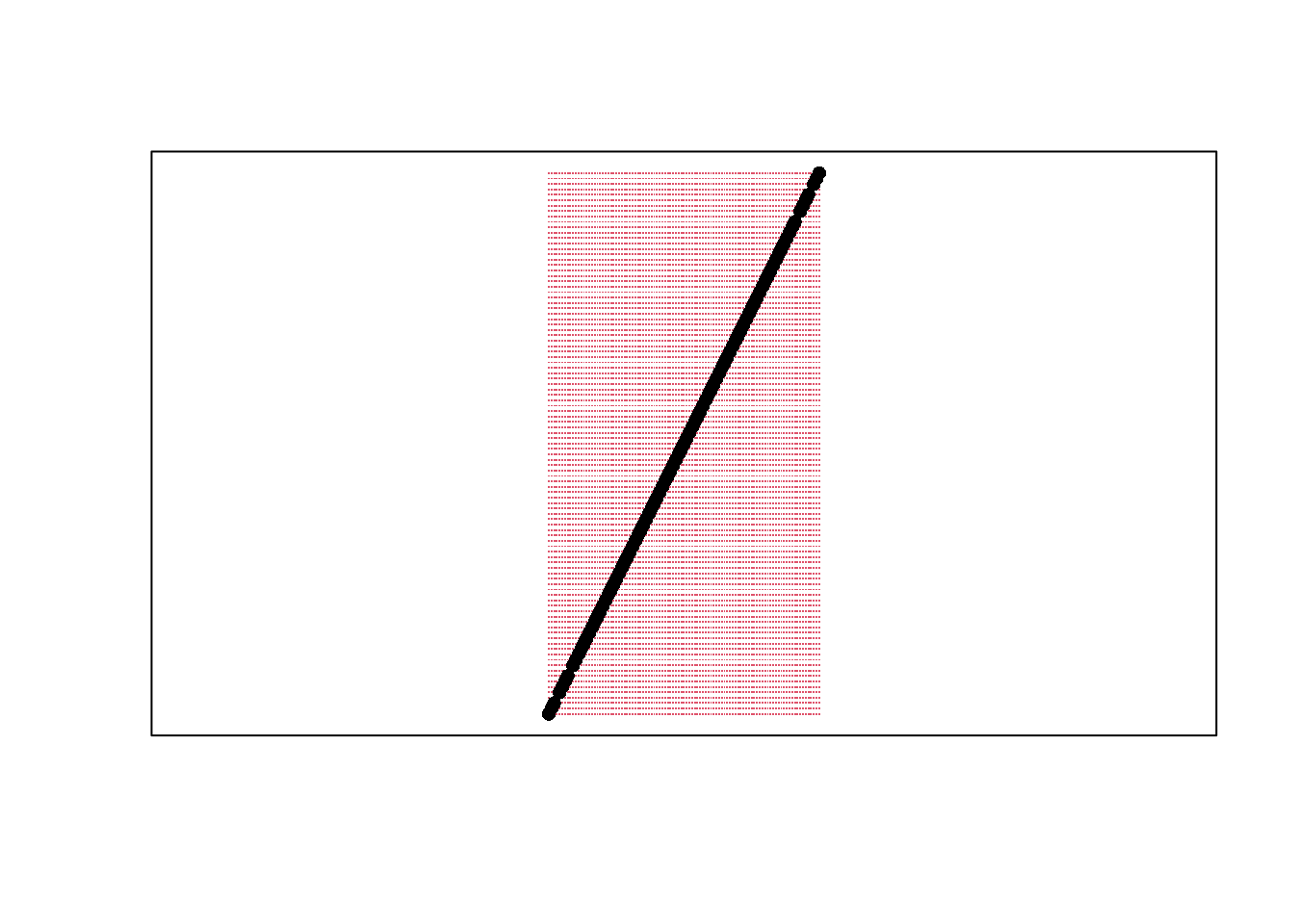
11.3 Posters and Slides
See
And download source files
Simply change the name to your own, and compile the document. If you have not installed Latex, then you must do that or specify a different output in order to compile DataScientism_Slides. For example, simply change output: beamer_presentation to output: ioslides_presentation on line 6.
11.4 Getting help w/ R Markdown
For more guidance on how to create Rmarkdown documents, see
- https://github.com/rstudio/cheatsheets/blob/main/rmarkdown.pdf
- https://cran.r-project.org/web/packages/rmarkdown/vignettes/rmarkdown.html
- http://rmarkdown.rstudio.com
- https://bookdown.org/yihui/rmarkdown/
- https://bookdown.org/yihui/rmarkdown-cookbook/
- https://dept.stat.lsa.umich.edu/~jerrick/courses/stat701/notes/rmarkdown.html
- An Introduction to the Advanced Theory and Practice of Nonparametric Econometrics. Raccine 2019. Appendices B & D.
- https://rmd4sci.njtierney.com/using-rmarkdown.html
If you are still lost, try one of the many online tutorials (such as these)
- https://www.rstudio.com/wp-content/uploads/2015/03/rmarkdown-reference.pdf
- https://github.com/adam-p/markdown-here/wiki/Markdown-Cheatsheet
- https://www.neonscience.org/resources/learning-hub/tutorials/rmd-code-intro
- https://m-clark.github.io/Introduction-to-Rmarkdown/
- https://www.stat.cmu.edu/~cshalizi/rmarkdown/
- http://math.wsu.edu/faculty/xchen/stat412/HwWriteUp.Rmd
- http://math.wsu.edu/faculty/xchen/stat412/HwWriteUp.html
- https://holtzy.github.io/Pimp-my-rmd/
- https://ntaback.github.io/UofT_STA130/Rmarkdownforclassreports.html
- https://crd150.github.io/hw_guidelines.html
- https://r4ds.had.co.nz/r-markdown.html
- http://www.stat.cmu.edu/~cshalizi/rmarkdown
- http://www.ssc.wisc.edu/sscc/pubs/RFR/RFR_RMarkdown.html
- http://kbroman.org/knitr_knutshell/pages/Rmarkdown.html