12 Multivariate Data
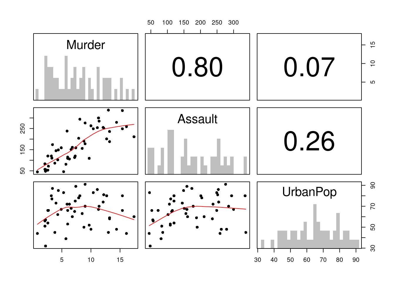
Given a dataset, you can summarize it using the previous tools.
##            Murder Assault UrbanPop Rape
## Alabama      13.2     236       58 21.2
## Alaska       10.0     263       48 44.5
## Arizona       8.1     294       80 31.0
## Arkansas      8.8     190       50 19.5
## California    9.0     276       91 40.6
## Colorado 7.9 204 78 38.7library(psych)
pairs.panels( USArrests[,c('Murder','Assault','UrbanPop')],
hist.col=grey(0,.25), breaks=30, density=F, hist.border=NA, # Diagonal
ellipses=F, rug=F, smoother=F, pch=16, col='red' # Lower Triangle
)
12.1 Multiple Linear Regression
With \(K\) variables, the linear model is \[ y_i=\beta_0+\beta_1 x_{i1}+\beta_2 x_{i2}+\ldots+\beta_K x_{iK}+\epsilon_i = [1~~ x_{i1} ~~...~~ x_{iK}] \beta + \epsilon_i \] and our objective is \[ min_{\beta} \sum_{i=1}^{N} (\epsilon_i)^2. \]
Denoting \[ y= \begin{pmatrix} y_{1} \\ \vdots \\ y_{N} \end{pmatrix} \quad \textbf{X} = \begin{pmatrix} 1 & x_{11} & ... & x_{1K} \\ & \vdots & & \\ 1 & x_{N1} & ... & x_{NK} \end{pmatrix}, \] we can also write the model and objective in matrix form \[ y=\textbf{X}\beta+\epsilon\\ min_{\beta} (\epsilon' \epsilon) \]
Minimizing the squared errors yields coefficient estimates \[ \hat{\beta}=(\textbf{X}'\textbf{X})^{-1}\textbf{X}'y \] and predictions \[ \hat{y}=\textbf{X} \hat{\beta} \\ \hat{\epsilon}=y - \hat{y} \\ \]
# Manually Compute
Y <- USArrests[,'Murder']
X <- USArrests[,c('Assault','UrbanPop')]
X <- as.matrix(cbind(1,X))

XtXi <- solve(t(X)%*%X)
Bhat <- XtXi %*% (t(X)%*%Y)
c(Bhat)
## [1] 3.20715340 0.04390995 -0.04451047## (Intercept) Assault UrbanPop
## 3.20715340 0.04390995 -0.04451047To measure the ``Goodness of fit’’ of the model, we can again plot our predictions
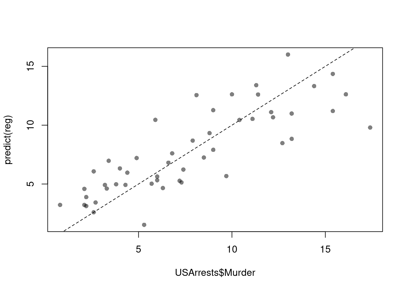 and compute sums of squared errors. Adding random data may sometimes improve the fit, however, so we adjust the \(R^2\) by the number of covariates \(K\).
\[
R^2 = \frac{ESS}{TSS}=1-\frac{RSS}{TSS}\\
R^2_{\text{adj.}} = 1-\frac{N-1}{N-K}(1-R^2)
\]
and compute sums of squared errors. Adding random data may sometimes improve the fit, however, so we adjust the \(R^2\) by the number of covariates \(K\).
\[
R^2 = \frac{ESS}{TSS}=1-\frac{RSS}{TSS}\\
R^2_{\text{adj.}} = 1-\frac{N-1}{N-K}(1-R^2)
\]
ksims <- 1:30
for(k in ksims){
    USArrests[,paste0('R',k)] <- runif(nrow(USArrests),0,20)
}
reg_sim <- lapply(ksims, function(k){
    rvars <- c('Assault','UrbanPop', paste0('R',1:k))
    rvars2 <- paste0(rvars, collapse='+')
    reg_k <- lm( paste0('Murder~',rvars2), data=USArrests)
})
R2_sim <- sapply(reg_sim, function(reg_k){  summary(reg_k)$r.squared })
R2adj_sim <- sapply(reg_sim, function(reg_k){  summary(reg_k)$adj.r.squared })

plot.new()
plot.window(xlim=c(0,30), ylim=c(0,1))
points(ksims, R2_sim)
points(ksims, R2adj_sim, pch=16)
axis(1)
axis(2)
mtext(expression(R^2),2, line=3)
mtext('Additional Random Covariates', 1, line=3)
legend('topleft', horiz=T,
    legend=c('Undjusted', 'Adjusted'), pch=c(1,16))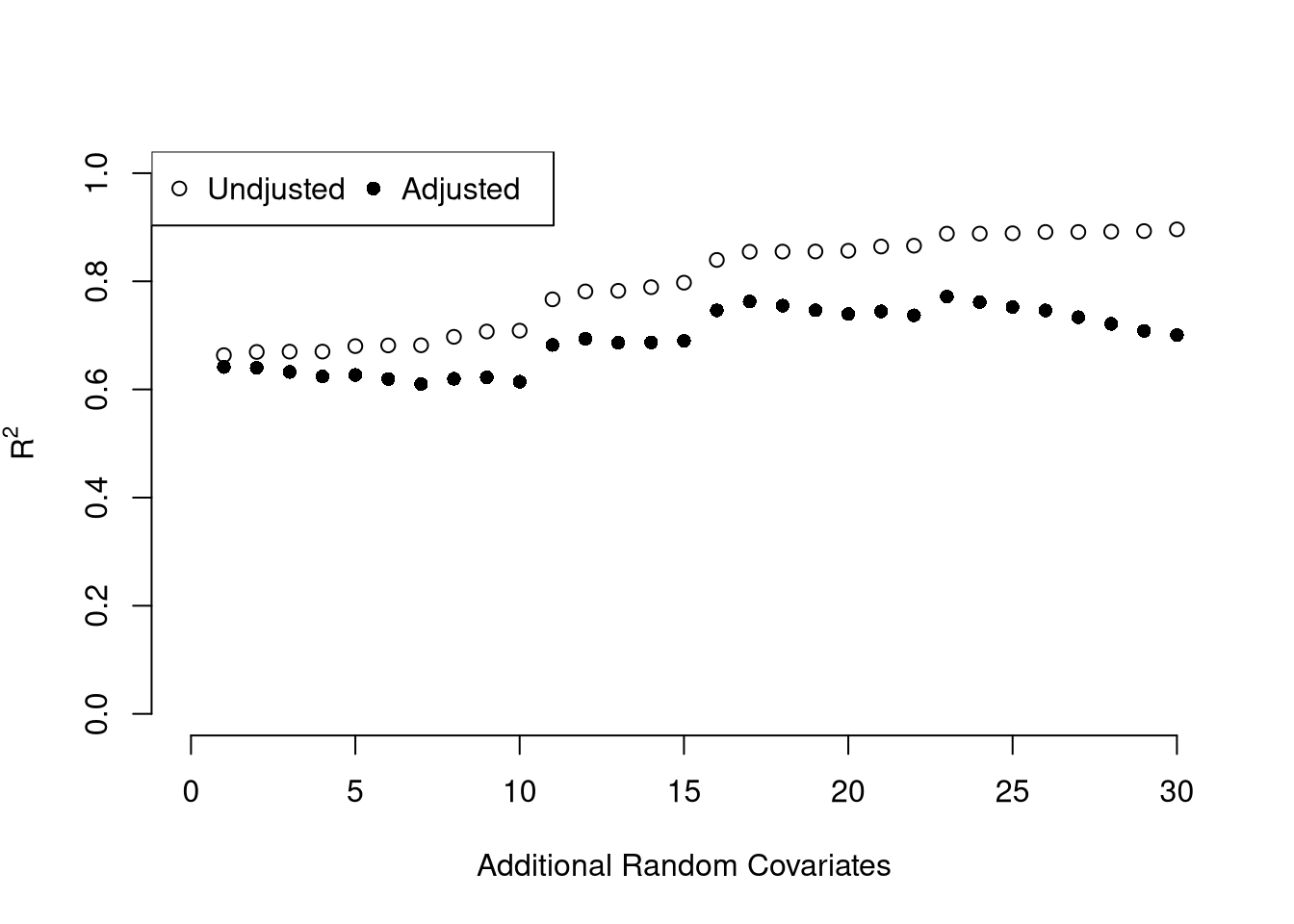
12.2 Variability and Hypothesis Tests
To estimate the variability of our estimates, we can use the same data-driven methods introduced in the last section. As before, we can conduct independent hypothesis tests using t-values.
We can also conduct joint tests that account for interdependancies in our estimates. For example, to test whether two coefficients both equal \(0\), we bootstrap the joint distribution of coefficients.
# Bootstrap SE's
boots <- 1:399
boot_regs <- lapply(boots, function(b){
    b_id <- sample( nrow(USArrests), replace=T)
    xy_b <- USArrests[b_id,]
    reg_b <- lm(Murder~Assault+UrbanPop, dat=xy_b)
})
boot_coefs <- sapply(boot_regs, coef)

# Recenter at 0 to impose the null
#boot_means <- rowMeans(boot_coefs)
#boot_coefs0 <- sweep(boot_coefs, MARGIN=1, STATS=boot_means)
boot_coef_df <- as.data.frame(cbind(ID=boots, t(boot_coefs)))
fig <- plotly::plot_ly(boot_coef_df,
type = 'scatter', mode = 'markers',
x = ~UrbanPop, y = ~Assault,
text = ~paste('<b> bootstrap dataset: ', ID, '</b>',
'<br>Coef. Urban :', round(UrbanPop,3),
'<br>Coef. Murder :', round(Assault,3),
'<br>Coef. Intercept :', round(`(Intercept)`,3)),
hoverinfo='text',
showlegend=F,
marker=list( color='rgba(0, 0, 0, 0.5)'))
fig <- plotly::layout(fig,
showlegend=F,
title='Joint Distribution of Coefficients (under the null)',
xaxis = list(title='UrbanPop Coefficient'),
yaxis = list(title='Assualt Coefficient'))
figF-statistic.
We can also use an \(F\) test for any \(q\) hypotheses. Specifically, when \(q\) hypotheses restrict a model, the degrees of freedom drop from \(k_{u}\) to \(k_{r}\) and the residual sum of squares \(RSS=\sum_{i}(y_{i}-\widehat{y}_{i})^2\) typically increases. We compute the statistic \[ F_{q} = \frac{(RSS_{r}-RSS_{u})/(k_{u}-k_{r})}{RSS_{u}/(N-k_{u})} \]
If you test whether all \(K\) variables are significant, the restricted model is a simple intercept and \(RSS_{r}=TSS\), and \(F_{q}\) can be written in terms of \(R^2\): \(F_{K} = \frac{R^2}{1-R^2} \frac{N-K}{K-1}\). The first fraction is the relative goodness of fit, and the second fraction is an adjustment for degrees of freedom (similar to how we adjusted the \(R^2\) term before).
To conduct a hypothesis test, first compute a null distribution by randomly reshuffling the outcomes and recompute the \(F\) statistic, and then compare how often random data give something as extreme as your initial statistic. For some intuition on this F test, examine how the adjusted \(R^2\) statistic varies with bootstrap samples.
# Bootstrap under the null
boots <- 1:399
boot_regs0 <- lapply(boots, function(b){
  # Generate bootstrap sample
  xy_b <- USArrests
  b_id <- sample( nrow(USArrests), replace=T)
  # Impose the null
  xy_b$Murder <-  xy_b$Murder[b_id]
  # Run regression
  reg_b <- lm(Murder~Assault+UrbanPop, dat=xy_b)
})
# Get null distribution for adjusted R2
R2adj_sim0 <- sapply(boot_regs0, function(reg_k){
    summary(reg_k)$adj.r.squared })
hist(R2adj_sim0, xlim=c(-.1,1), breaks=25, border=NA,
    main='', xlab=expression('adj.'~R[b]^2))

# Compare to initial statistic
abline(v=summary(reg)$adj.r.squared, lwd=2, col=2)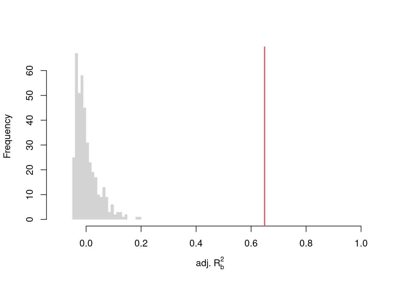
Note that hypothesis testing is not to be done routinely, as additional complications arise when testing multiple hypothesis sequentially.
Under some additional assumptions \(F_{q}\) follows an F-distribution. For more about F-testing, see https://online.stat.psu.edu/stat501/lesson/6/6.2 and https://www.econometrics.blog/post/understanding-the-f-statistic/
12.3 Factor Variables
So far, we have discussed cardinal data where the difference between units always means the same thing: e.g., \(4-3=2-1\). There are also factor variables
- Ordered: refers to Ordinal data. The difference between units means something, but not always the same thing. For example, \(4th - 3rd \neq 2nd - 1st\).
- Unordered: refers to Categorical data. The difference between units is meaningless. For example, \(B-A=?\)
To analyze either factor, we often convert them into indicator variables or dummies; \(D_{c}=\mathbf{1}( Factor = c)\). One common case is if you have observations of individuals over time periods, then you may have two factor variables. An unordered factor that indicates who an individual is; for example \(D_{i}=\mathbf{1}( Individual = i)\), and an order factor that indicates the time period; for example \(D_{t}=\mathbf{1}( Time \in [month~ t, month~ t+1) )\). There are many other cases you see factor variables, including spatial ID’s in purely cross sectional data.
Be careful not to handle categorical data as if they were cardinal. E.g., generate city data with Leipzig=1, Lausanne=2, LosAngeles=3, … and then include city as if it were a cardinal number (that’s a big no-no). The same applied to ordinal data; PopulationLeipzig=2, PopulationLausanne=3, PopulationLosAngeles=1.
N <- 1000
x <- runif(N,3,8)
e <- rnorm(N,0,0.4)
fo <- factor(rbinom(N,4,.5), ordered=T)
fu <- factor(rep(c('A','B'),N/2), ordered=F)
dA <- 1*(fu=='A')
y <- (2^as.integer(fo)*dA )*sqrt(x)+ 2*as.integer(fo)*e
dat_f <- data.frame(y,x,fo,fu)
With factors, you can still include them in the design matrix of an OLS regression \[ y_{it} = x_{it} \beta_{x} + d_{t}\beta_{t} \] When, as commonly done, the factors are modeled as being additively seperable, they are modeled “fixed effects”.5 Simply including the factors into the OLS regression yields a “dummy variable” fixed effects estimator. Hansen Econometrics, Theorem 17.1: The fixed effects estimator of \(\beta\) algebraically equals the dummy variable estimator of \(\beta\). The two estimators have the same residuals.
##        x
## 1.202273## $fo
## 0 1 2 3 4
## 6.770865 9.020095 14.148339 22.655792 44.346932
##
## $fu
## A B
## 0.00000 -23.14793## x fo0 fo1 fo2 fo3 fo4 fuB
## 1.202273 6.770865 9.020095 14.148339 22.655792 44.346932 -23.147928With fixed effects, we can also compute averages for each group and construct a between estimator: \(\bar{y}_i = \alpha + \bar{x}_i \beta\). Or we can subtract the average from each group to construct a within estimator: \((y_{it} - \bar{y}_i) = (x_{it}-\bar{x}_i)\beta\).
But note that many factors are not additively separable. This is easy to check with an F-test;
reg0 <- lm(y~-1+x+fo+fu, dat_f)
reg1 <- lm(y~-1+x+fo*fu, dat_f)
reg2 <- lm(y~-1+x*fo*fu, dat_f)

anova(reg0, reg2)
## Analysis of Variance Table
##
## Model 1: y ~ -1 + x + fo + fu
## Model 2: y ~ -1 + x * fo * fu
## Res.Df RSS Df Sum of Sq F Pr(>F)
## 1 993 80781
## 2 980 5754 13 75028 983 < 2.2e-16 ***
## ---
## Signif. codes: 0 '***' 0.001 '**' 0.01 '*' 0.05 '.' 0.1 ' ' 1## Analysis of Variance Table
##
## Model 1: y ~ -1 + x + fo + fu
## Model 2: y ~ -1 + x + fo * fu
## Model 3: y ~ -1 + x * fo * fu
## Res.Df RSS Df Sum of Sq F Pr(>F)
## 1 993 80781
## 2 989 11361 4 69421 2956.01 < 2.2e-16 ***
## 3 980 5754 9 5607 106.11 < 2.2e-16 ***
## ---
## Signif. codes: 0 '***' 0.001 '**' 0.01 '*' 0.05 '.' 0.1 ' ' 1Break Points. Kinks and Discontinuities in \(X\) can also be modeled using factor variables. As such, \(F\)-tests can be used to examine whether a breaks is statistically significant.
library(AER); data(CASchools)
CASchools$score <- (CASchools$read + CASchools$math) / 2
reg <- lm(score~income, data=CASchools)

# F Test for Break
reg2 <- lm(score ~ income*I(income>15), data=CASchools)
anova(reg, reg2)

# Chow Test for Break
data_splits <- split(CASchools, CASchools$income <= 15)
resids <- sapply(data_splits, function(dat){
    reg <- lm(score ~ income, data=dat)
    sum( resid(reg)^2)
})
Ns <-  sapply(data_splits, function(dat){ nrow(dat)})
Rt <- (sum(resid(reg)^2) - sum(resids))/sum(resids)
Rb <- (sum(Ns)-2*reg$rank)/reg$rank
Ft <- Rt*Rb
pf(Ft,reg$rank, sum(Ns)-2*reg$rank,lower.tail=F)

# See also
# strucchange::sctest(y~x, data=xy, type="Chow", point=.5)
# strucchange::Fstats(y~x, data=xy)

# To Find Changes
# segmented::segmented(reg)
12.4 Coefficient Interpretation
Notice that we have gotten pretty far without actually trying to meaningfully interpret regression coefficients. That is because the above procedure will always give us number, regardless as to whether the true data generating process is linear or not. So, to be cautious, we have been interpreting the regression outputs while being agnostic as to how the data are generated. We now consider a special situation where we know the data are generated according to a linear process and are only uncertain about the parameter values.
If the data generating process is \[ y=X\beta + \epsilon\\ \mathbb{E}[\epsilon | X]=0, \] then we have a famous result that lets us attach a simple interpretation of OLS coefficients as unbiased estimates of the effect of X: \[ \hat{\beta} = (X'X)^{-1}X'y = (X'X)^{-1}X'(X\beta + \epsilon) = \beta + (X'X)^{-1}X'\epsilon\\ \mathbb{E}\left[ \hat{\beta} \right] = \mathbb{E}\left[ (X'X)^{-1}X'y \right] = \beta + (X'X)^{-1}\mathbb{E}\left[ X'\epsilon \right] = \beta \]
Generate a simulated dataset with 30 observations and two exogenous variables. Assume the following relationship: \(y_{i} = \beta_0 + \beta_1 x_{i1} + \beta_2 x_{i2} + \epsilon_i\) where the variables and the error term are realizations of the following data generating processes (DGP):
N <- 30
B <- c(10, 2, -1)

x1 <- runif(N, 0, 5)
x2 <- rbinom(N,1,.7)
X <- cbind(1,x1,x2)
e <- rnorm(N,0,3)
Y <- X%*%B + e
dat <- data.frame(Y,X)
coef(lm(Y~x1+x2, data=dat))
## (Intercept) x1 x2
## 10.375993 1.850176 -1.301420Simulate the distribution of coefficients under a correctly specified model. Interpret the average.
N <- 30
B <- c(10, 2, -1)

Coefs <- sapply(1:400, function(sim){
    x1 <- runif(N, 0, 5)
    x2 <- rbinom(N,1,.7)
    X <- cbind(1,x1,x2)
    e <- rnorm(N,0,3)
    Y <- X%*%B + e
    dat <- data.frame(Y,x1,x2)
    coef(lm(Y~x1+x2, data=dat))
})

par(mfrow=c(1,2))
for(i in 2:3){
    hist(Coefs[i,], xlab=bquote(beta[.(i)]), main='', border=NA)
    abline(v=mean(Coefs[i,]), lwd=2)
    abline(v=B[i], col=rgb(1,0,0))
}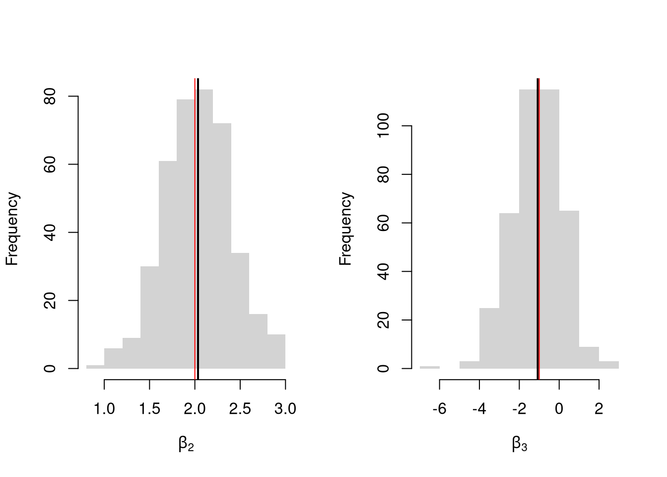
Many economic phenomena are nonlinear, even when including potential transforms of \(Y\) and \(X\). Sometimes the linear model may still be a good or even great approximation. But sometimes not, and it is hard to know ex-ante. Examine the distribution of coefficients under this mispecified model and try to interpret the average.
N <- 30

Coefs <- sapply(1:600, function(sim){
    x2 <- runif(N, 0, 5)
    x3 <- rbinom(N,1,.7)
    e <- rnorm(N,0,3)
    Y <- 10*x3 + 2*log(x2)^x3 + e
    dat <- data.frame(Y,x2,x3)
    coef(lm(Y~x2+x3, data=dat))
})

par(mfrow=c(1,2))
for(i in 2:3){
    hist(Coefs[i,],  xlab=bquote(beta[.(i)]), main='', border=NA)
    abline(v=mean(Coefs[i,]), col=1, lwd=2)
}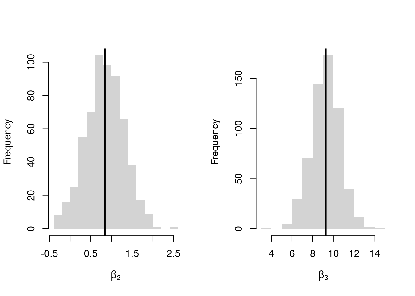
In general, you can interpret your regression coefficients as “adjusted correlations”. There are (many) tests for whether the relationships in your dataset are actually additively separable and linear.
12.5 Transformations
Transforming variables can often improve your model fit while still allowing it estimated via OLS. This is because OLS only requires the model to be linear in the parameters. Under the assumptions of the model is correctly specified, the following table is how we can interpret the coefficients of the transformed data. (Note for small changes, \(\Delta ln(x) \approx \Delta x / x = \Delta x \% \cdot 100\).)
| Specification | Regressand | Regressor | Derivative | Interpretation (If True) |
|---|---|---|---|---|
| linear–linear | \(y\) | \(x\) | \(\Delta y = \beta_1\cdot\Delta x\) | Change \(x\) by one unit \(\rightarrow\) change \(y\) by \(\beta_1\) units. |
| log–linear | \(ln(y)\) | \(x\) | \(\Delta y \% \cdot 100 \approx \beta_1 \cdot \Delta x\) | Change \(x\) by one unit \(\rightarrow\) change \(y\) by \(100 \cdot \beta_1\) percent. |
| linear–log | \(y\) | \(ln(x)\) | \(\Delta y \approx \frac{\beta_1}{100}\cdot \Delta x \%\) | Change \(x\) by one percent \(\rightarrow\) change \(y\) by \(\frac{\beta_1}{100}\) units |
| log–log | \(ln(y)\) | \(ln(x)\) | \(\Delta y \% \approx \beta_1\cdot \Delta x \%\) | Change \(x\) by one percent \(\rightarrow\) change \(y\) by \(\beta_1\) percent |
Now recall from micro theory that an additively seperable and linear production function is referred to as ``perfect substitutes’‘. With a linear model and untranformed data, you have implicitly modelled the different regressors \(X\) as perfect substitutes. Further recall that the’‘perfect substitutes’’ model is a special case of the constant elasticity of substitution production function. Here, we will build on http://dx.doi.org/10.2139/ssrn.3917397, and consider box-cox transforming both \(X\) and \(y\). Specifically, apply the box-cox transform of \(y\) using parameter \(\lambda\) and apply another box-cox transform to each \(x\) using the same parameter \(\rho\) so that \[ y^{(\lambda)}_{i} = \sum_{k=1}^{K}\beta_{k} x^{(\rho)}_{ik} + \epsilon_{i}\\ y^{(\lambda)}_{i} = \begin{cases} \lambda^{-1}[ (y_i+1)^{\lambda}- 1] & \lambda \neq 0 \\ log(y_i+1) & \lambda=0 \end{cases}.\\ x^{(\rho)}_{i} = \begin{cases} \rho^{-1}[ (x_i)^{\rho}- 1] & \rho \neq 0 \\ log(x_{i}+1) & \rho=0 \end{cases}. \]
Notice that this nests:
- linear-linear \((\rho=\lambda=1)\).
- linear-log \((\rho=1, \lambda=0)\).
- log-linear \((\rho=0, \lambda=1)\).
- log-log \((\rho=\lambda=0)\).
If \(\rho=\lambda\), we get the CES production function. This nests the ‘’perfect substitutes’’ linear-linear model (\(\rho=\lambda=1\)) , the ‘’cobb-douglas’’ log-log model (\(\rho=\lambda=0\)), and many others. We can define \(\lambda=\rho/\lambda'\) to be clear that this is indeed a CES-type transformation where
- \(\rho \in (-\infty,1]\) controls the “substitutability” of explanatory variables. E.g., \(\rho <0\) is ‘’complementary’’.
- \(\lambda\) determines ‘’returns to scale’‘. E.g., \(\lambda<1\) is’‘decreasing returns’’.
We compute the mean squared error in the original scale by inverting the predictions; \[ \widehat{y}_{i} = \begin{cases} [ \widehat{y}_{i}^{(\lambda)} \cdot \lambda ]^{1/\lambda} -1 & \lambda \neq 0 \\ exp( \widehat{y}_{i}^{(\lambda)}) -1 & \lambda=0 \end{cases}. \]
It is easiest to optimize parameters in a 2-step procedure called `concentrated optimization’. We first solve for \(\widehat{\beta}(\rho,\lambda)\) and compute the mean squared error \(MSE(\rho,\lambda)\). We then find the \((\rho,\lambda)\) which minimizes \(MSE\).
# Box-Cox Transformation Function
bxcx <- function( xy, rho){
    if (rho == 0L) {
      log(xy+1)
    } else if(rho == 1L){
      xy
    } else {
      ((xy+1)^rho - 1)/rho
    }
}
bxcx_inv <- function( xy, rho){
    if (rho == 0L) {
      exp(xy) - 1
    } else if(rho == 1L){
      xy
    } else {
     (xy * rho + 1)^(1/rho) - 1
    }
}

# Which Variables
reg <- lm(Murder~Assault+UrbanPop, data=USArrests)
X <- USArrests[,c('Assault','UrbanPop')]
Y <- USArrests[,'Murder']

# Simple Grid Search over potential (Rho,Lambda)
rl_df <- expand.grid(rho=seq(-2,2,by=.5),lambda=seq(-2,2,by=.5))

# Compute Mean Squared Error
# from OLS on Transformed Data
errors <- apply(rl_df,1,function(rl){
    Xr <- bxcx(X,rl[[1]])
    Yr <- bxcx(Y,rl[[2]])
    Datr <- cbind(Murder=Yr,Xr)
    Regr <- lm(Murder~Assault+UrbanPop, data=Datr)
    Predr <- bxcx_inv(predict(Regr),rl[[2]])
    Resr  <- (Y - Predr)
    return(Resr)
})
rl_df$mse <- colMeans(errors^2)

# Want Small MSE and Interpretable
layout(matrix(1:2,ncol=2), width=c(3,1), height=c(1,1))
par(mar=c(4,4,2,0))
plot(lambda~rho,rl_df, cex=8, pch=15,
    xlab=expression(rho),
    ylab=expression(lambda),
    col=hcl.colors(25)[cut(1/rl_df$mse,25)])
# Which min
rl0 <- rl_df[which.min(rl_df$mse),c('rho','lambda')]
points(rl0$rho, rl0$lambda, pch=0, col=1, cex=8, lwd=2)
# Legend
plot(c(0,2),c(0,1), type='n', axes=F,
    xlab='',ylab='', cex.main=.8,
    main=expression(frac(1,'Mean Square Error')))
rasterImage(as.raster(matrix(hcl.colors(25), ncol=1)), 0, 0, 1,1)
text(x=1.5, y=seq(1,0,l=10), cex=.5,
    labels=levels(cut(1/rl_df$mse,10)))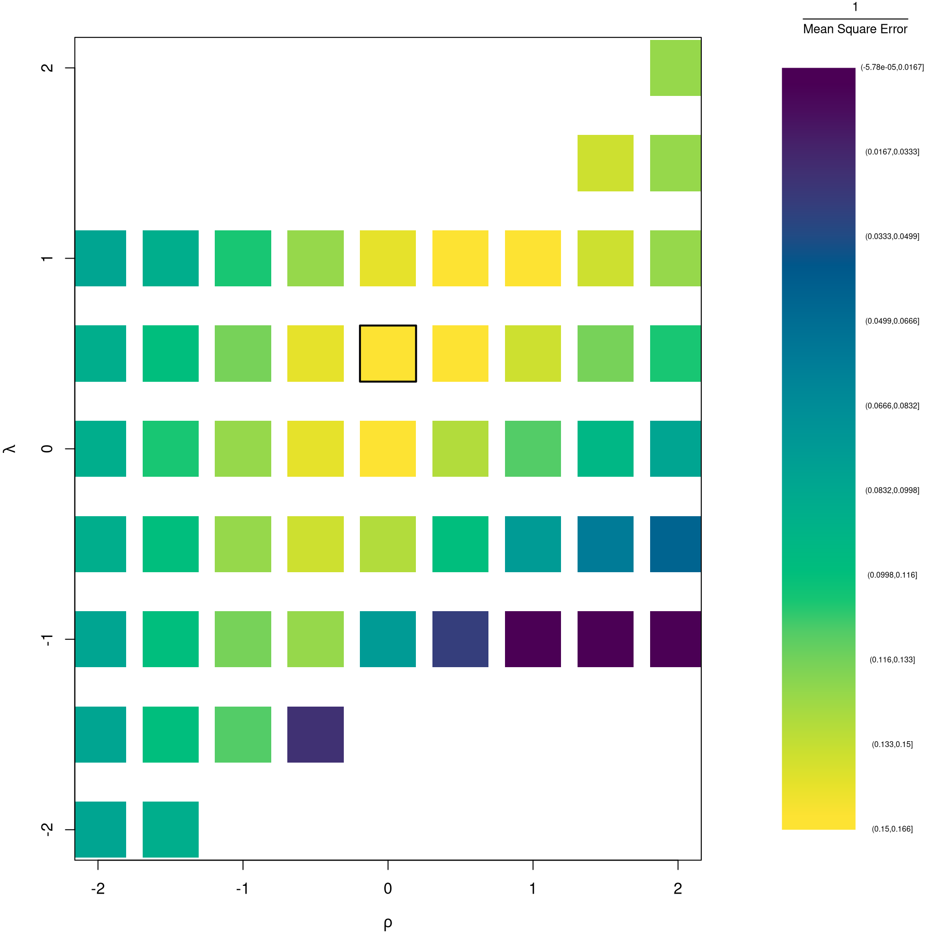
The parameters \(-1,0,1,2\) are easy to interpret and might be selected instead if there is only a small loss in fit. (In the above example, we might choose \(\lambda=0\) instead of the \(\lambda\) which minimized the mean square error). You can also plot the specific predictions to better understand the effect of data transformation beyond mean squared error.
# Plot for Specific Comparisons
Xr <- bxcx(X,rl0[[1]])
Yr <- bxcx(Y,rl0[[2]])
Datr <- cbind(Murder=Yr,Xr)
Regr <- lm(Murder~Assault+UrbanPop, data=Datr)
Predr <- bxcx_inv(predict(Regr),rl0[[2]])

cols <- c(rgb(1,0,0,.5), col=rgb(0,0,1,.5))
plot(Y, Predr, pch=16, col=cols[1], ylab='Prediction',
    ylim=range(Y,Predr))
points(Y, predict(reg), pch=16, col=cols[2])
legend('topleft', pch=c(16), col=cols,
    title=expression(rho~', '~lambda),
    legend=c(  paste0(rl0, collapse=', '),'1, 1') )
abline(a=0,b=1, lty=2)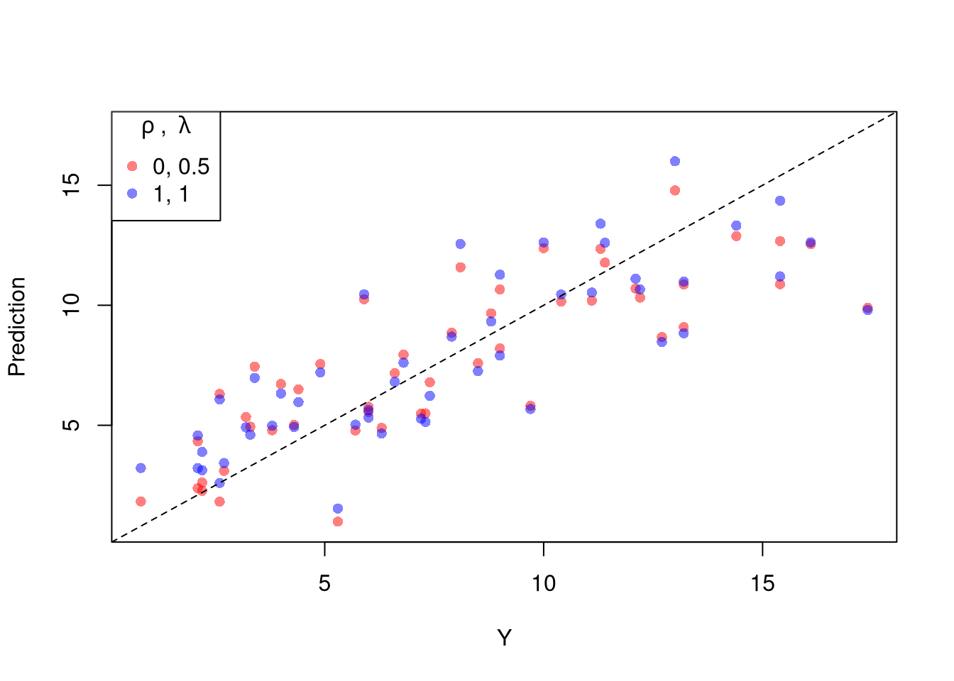
When explicitly transforming data according to \(\lambda\) and \(\rho\), these parameters increase the degrees of freedom by two. The default hypothesis testing procedures do not account for you trying out different transformations, and should be adjusted by the increased degrees of freedom. Specification searches deflate standard errors and are a major source for false discoveries.
12.6 Diagnostics
There’s little sense in getting great standard errors for a terrible model. Plotting your regression object a simple and easy step to help diagnose whether your model is in some way bad. We next go through what each of these figures show.
reg <- lm(Murder~Assault+UrbanPop, data=USArrests)
par(mfrow=c(2,2))
plot(reg, pch=16, col=grey(0,.5))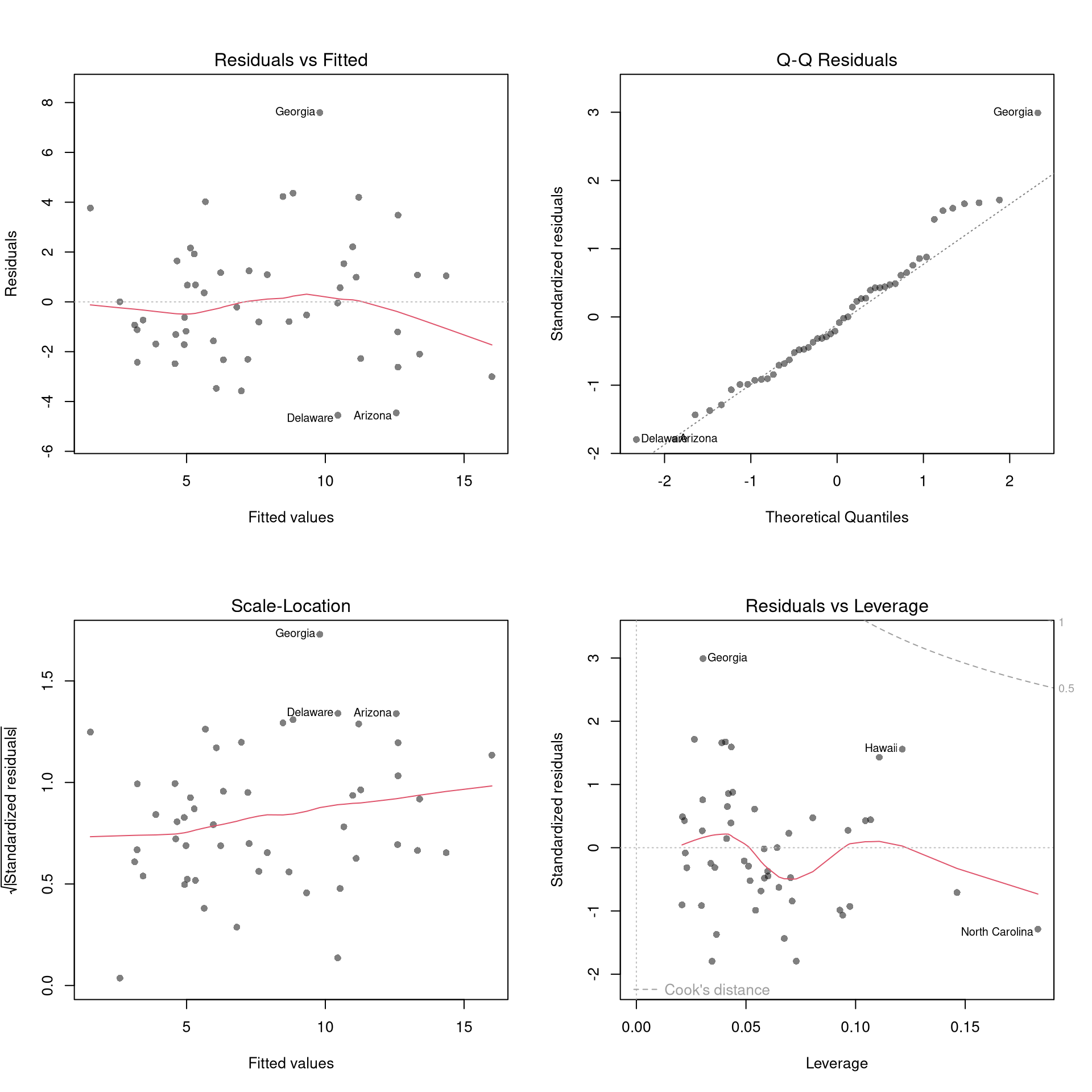
Outliers. The first diagnostic plot examines outliers in terms the outcome \(y_i\) being far from its prediction \(\hat{y}_i\). You may be interested in such outliers because they can (but do not have to) unduly influence your estimates.
The third diagnostic plot examines another type of outlier, where an observation with the explanatory variable \(x_i\) is far from the center of mass of the other \(x\)’s. A point has high leverage if the estimates change dramatically when you estimate the model without that data point.
N <- 40
x <- c(25, runif(N-1,3,8))
e <- rnorm(N,0,0.4)
y <- 3 + 0.6*sqrt(x) + e
plot(y~x, pch=16, col=grey(0,.5))
points(x[1],y[1], pch=16, col=rgb(1,0,0,.5))

abline(lm(y~x), col=2, lty=2)
abline(lm(y[-1]~x[-1]))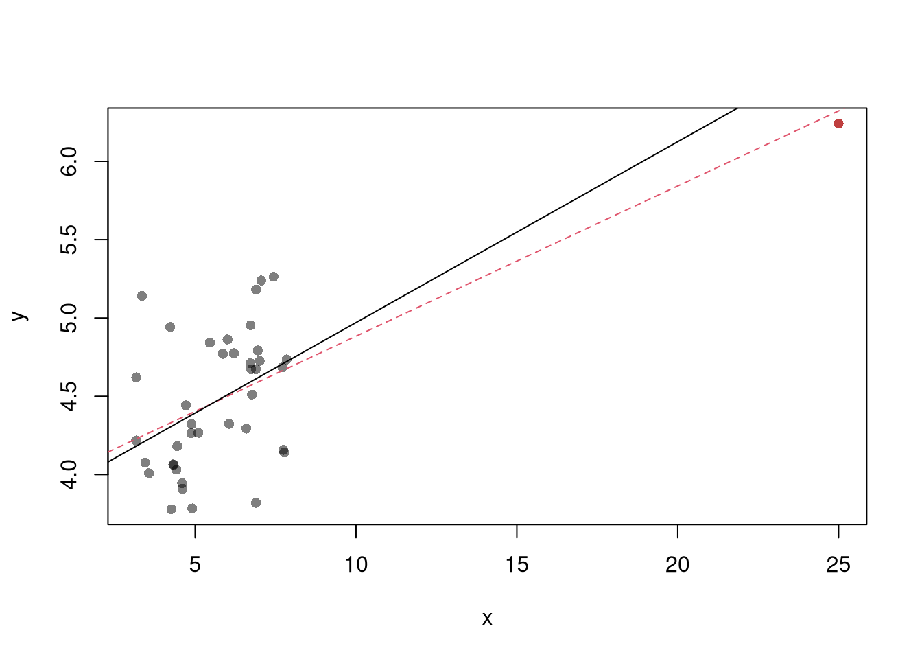
See AEJ-leverage and NBER-leverage for examples of leverage in economics.
Standardized residuals are \[ r_i=\frac{\hat{\epsilon}_i}{s_{[i]}\sqrt{1-h_i}}, \] where \(s_{[i]}\) is the root mean squared error of a regression with the \(i\)th observation removed and \(h_i\) is the leverage of residual \(\hat{\epsilon_i}\).
(See https://www.r-bloggers.com/2016/06/leverage-and-influence-in-a-nutshell/ for a good interactive explanation, and https://online.stat.psu.edu/stat462/node/87/ for detail.)
The fourth plot further assesses outlier \(X\) using Cook’s Distance, which sums of all prediction changes when observation i is removed and scales proportionally to the mean square error \(s^2 = \frac{\sum_{i} (e_{i})^2 }{n-K}.\)$ D_{i} = = $$
Normality. The second plot examines whether the residuals are normally distributed. Your OLS coefficient estimates do not depend on the normality of the residuals. (Good thing, because there’s no reason the residuals of economic phenomena should be so well behaved.) Many hypothesis tests are, however, affected by the distribution of the residuals. For these reasons, you may be interested in assessing normality
par(mfrow=c(1,2))
hist(resid(reg), main='Histogram of Residuals',
    font.main=1, border=NA)

qqnorm(resid(reg), main="Normal Q-Q Plot of Residuals",
    font.main=1, col=grey(0,.5), pch=16)
qqline(resid(reg), col=1, lty=2)

#shapiro.test(resid(reg))
Heterskedasticity may also matters for variability estimates. This is not shown in the plot, but you can conduct a simple test
Collinearity. This is when one explanatory variable in a multiple linear regression model can be linearly predicted from the others with a substantial degree of accuracy. Coefficient estimates may change erratically in response to small changes in the model or the data. (In the extreme case where there are more variables than observations \(K>N\), the inverse of \(X'X\) has an infinite number of solutions.) To diagnose collinearity, we can use the Variance Inflation Factor \[ VIF_{k}=\frac{1}{1-R^2_k}, \] where \(R^2_k\) is the \(R^2\) for the regression of \(X_k\) on the other covariates \(X_{-k}\) (a regression that does not involve the response variable Y)
12.7 More Literature
For OLS, see
- https://bookdown.org/josiesmith/qrmbook/linear-estimation-and-minimizing-error.html
- https://www.econometrics-with-r.org/4-lrwor.html
- https://www.econometrics-with-r.org/6-rmwmr.html
- https://www.econometrics-with-r.org/7-htaciimr.html
- https://bookdown.org/ripberjt/labbook/bivariate-linear-regression.html
- https://bookdown.org/ripberjt/labbook/multivariable-linear-regression.html
- https://online.stat.psu.edu/stat462/node/137/
- https://book.stat420.org/
- Hill, Griffiths & Lim (2007), Principles of Econometrics, 3rd ed., Wiley, S. 86f.
- Verbeek (2004), A Guide to Modern Econometrics, 2nd ed., Wiley, S. 51ff.
- Asteriou & Hall (2011), Applied Econometrics, 2nd ed., Palgrave MacMillan, S. 177ff.
- https://online.stat.psu.edu/stat485/lesson/11/
To derive OLS coefficients in Matrix form, see
- https://jrnold.github.io/intro-methods-notes/ols-in-matrix-form.html
- https://www.fsb.miamioh.edu/lij14/411_note_matrix.pdf
- https://web.stanford.edu/~mrosenfe/soc_meth_proj3/matrix_OLS_NYU_notes.pdf
For fixed effects, see
- https://www.econometrics-with-r.org/10-rwpd.html
- https://bookdown.org/josiesmith/qrmbook/topics-in-multiple-regression.html
- https://bookdown.org/ripberjt/labbook/multivariable-linear-regression.html
- https://www.princeton.edu/~otorres/Panel101.pdf
- https://www.stata.com/manuals13/xtxtreg.pdf
Diagnostics
- https://book.stat420.org/model-diagnostics.html#leverage
- https://socialsciences.mcmaster.ca/jfox/Books/RegressionDiagnostics/index.html
- https://bookdown.org/ripberjt/labbook/diagnosing-and-addressing-problems-in-linear-regression.html
- Belsley, D. A., Kuh, E., and Welsch, R. E. (1980). Regression Diagnostics: Identifying influential data and sources of collinearity. Wiley. https://doi.org/10.1002/0471725153
- Fox, J. D. (2020). Regression diagnostics: An introduction (2nd ed.). SAGE. https://dx.doi.org/10.4135/9781071878651
There are also random effects: the factor variable comes from a distribution that is uncorrelated with the regressors. This is rarely used in economics today, however, and are mostly included for historical reasons and special cases where fixed effects cannot be estimated due to data limitations.↩︎