6 (Re)Sampling

A sample is a subset of the population. A simple random sample is a sample where each possible sample of size n has the same probability of being selected.

Code

#All possible samples of two from {1,2,3,4}
#{1,2} {1,3}, {3,4}
#{2,3} {2,4}
#{3,4}
choose(4,2)
## [1] 6

# Random sample (no duplicates, equal probability)
sample(1:4, 2, replace=F)
## [1] 4 1

Sometimes, we can think of the population as being infinitely large. This is an approximation that makes mathematical calculations simpler.

Code

#All possible samples of two from an enormous bag of numbers {1,2,3,4}
#{1,1} {1,2} {1,3}, {3,4}
#{2,2} {2,3} {2,4}
#{3,3} {3,4}
#{4,4}

# Random sample (duplicates, equal probability)
sample(1:4, 2, replace=T)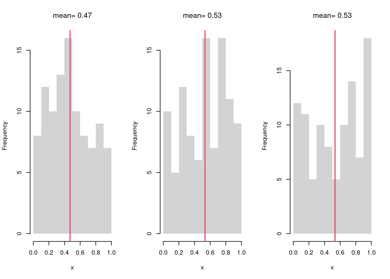
## [1] 2 3

6.1 Sample Distributions

The sampling distribution of a statistic shows us how much a statistic varies from sample to sample.

For example, see how the mean varies from sample to sample to sample.

Code

# Three Sample Example
par(mfrow=c(1,3))
for(i in 1:3){
    x <- runif(100) 
    m <-  mean(x)
    hist(x,
        breaks=seq(0,1,by=.1), #for comparability
        main=NA, border=NA)
    abline(v=m, col=2, lwd=2)
    title(paste0('mean= ', round(m,2)),  font.main=1)
}

Examine the sampling distribution of the mean

Code

sample_means <- sapply(1:1000, function(i){
    m <- mean(runif(100))
    return(m)
})
hist(sample_means, breaks=50, border=NA,
    col=2, font.main=1,
    main='Sampling Distribution of the mean')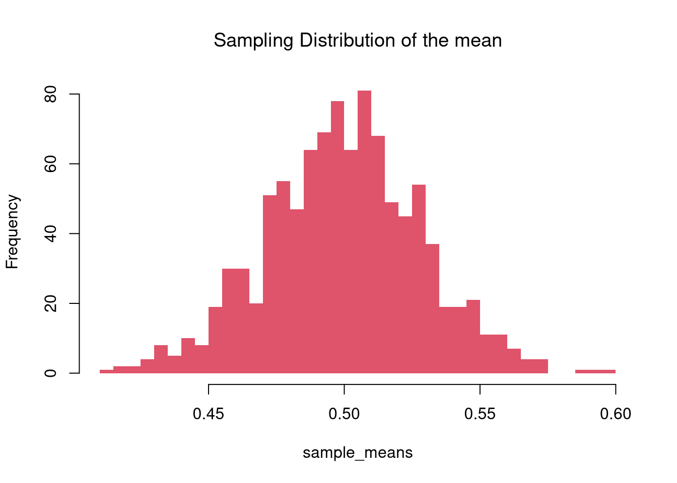

In this figure, you see two the most profound results known in statistics

Law of Large Numbers: the sample mean is centered around the true mean.
Central Limit Theorem: the sampling distribution of the mean is approximately standard normal.

Law of Large Numbers.

The Law of Large Numbers follows from Linearity of Expectations: the expected value of a sum of random variables is the sum of their individual expected values.

\[\begin{eqnarray} \mathbb{E}[X_{1}+X_{2}] &=&\mathbb{E}[X_{1}]+\mathbb{E}[X_{2}]\\ \mathbb{E}\left[\bar{X}\right] = \mathbb{E}\left[ \sum_{i=1}^{N} X_{i}/N \right] &=& \sum_{i=1}^{N} \mathbb{E}[X_{i}]/N. \end{eqnarray}\]

Assuming each data point has identical means; \(\mathbb{E}[X_{i}]=\mu\), the expected value of the sample average is the mean; \(\mathbb{E}\left[\bar{X}\right] = \sum_{i=1}^{N} \mu/N = \mu\).

See https://dlsun.github.io/probability/linearity.html

Central Limit Theorem.

There are actually many different variants of the central limit theorem (CLT): the sampling distribution of many statistics are standard normal. For example, examine the sampling distribution of the standard deviation.

Code

three_sds <- c(  sd(runif(100)),  sd(runif(100)),  sd(runif(100))  )
three_sds
## [1] 0.3021789 0.2889928 0.2822124

sample_sds <- sapply(1:1000, function(i){
    s <- sd(runif(100))
    return(s)
})
hist(sample_sds, breaks=50, border=NA,
    col=4, font.main=1,
    main='Sampling Distribution of the sd')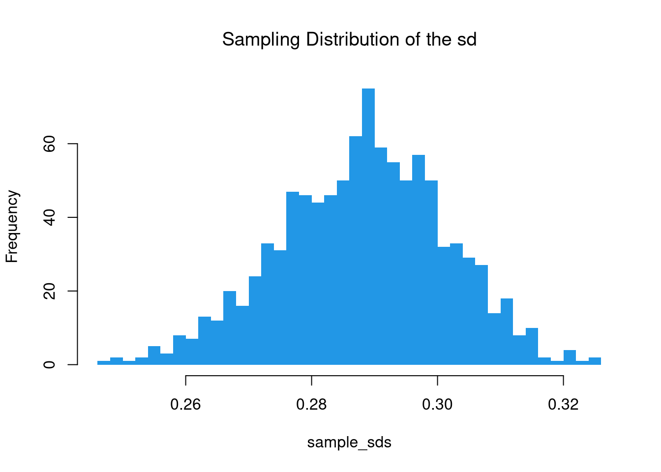

It is beyond this class to prove this result mathematically, but you should know that not all sampling distributions are standard normal.

The CLT does not apply to extremes. For example, examine which sampling distribution of the three main “order statistics” looks normal.

Code

# Create 300 samples, each with 1000 random uniform variables
x <- sapply(1:300, function(i) runif(1000) )
# Each row is a new sample
length(x[1,])
## [1] 300

# Median looks normal, Maximum and Minumum do not!
xmin <- apply(x,1, quantile, probs=0)
xmed <- apply(x,1, quantile, probs=.5)
xmax <- apply(x,1, quantile, probs=1)
par(mfrow=c(1,3))
hist(xmin, breaks=100, border=NA, main='Min', font.main=1)
hist(xmed, breaks=100, border=NA, main='Med', font.main=1)
hist(xmax, breaks=100, border=NA, main='Max', font.main=1)
title('Sampling Distributions', outer=T, line=-1)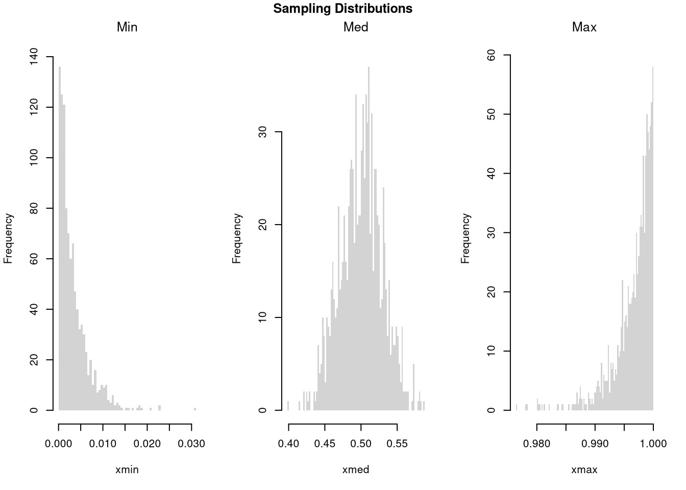

The CLT also assumes the variances are well behaved. For example,

Code

x <- sapply(1:400, function(i) rcauchy(1000,0,10) )
hist(colMeans(x), breaks=100, border=NA) # Tails look too "fat"

Code

# Explore any function!
fun_of_rv <- function(f, n=100){
  x <- runif(n) # modify to try a different random variable
  y <- f(x) 
  return(y)
}

fun_of_rv( f=mean )
## [1] 0.5053212

fun_of_rv( f=function(i){ diff(range(exp(i))) } )
## [1] 1.711343

6.2 Resampling

Often, we only have one sample. How then can we estimate the sampling distribution of a statistic?

Code

sample_dat <- USArrests[,'Murder']
mean(sample_dat)
## [1] 7.788

We can “resample” our data. Hesterberg (2015) provides a nice illustration of the idea. The two most basic versions are the jackknife and the bootstrap, which are discussed below.

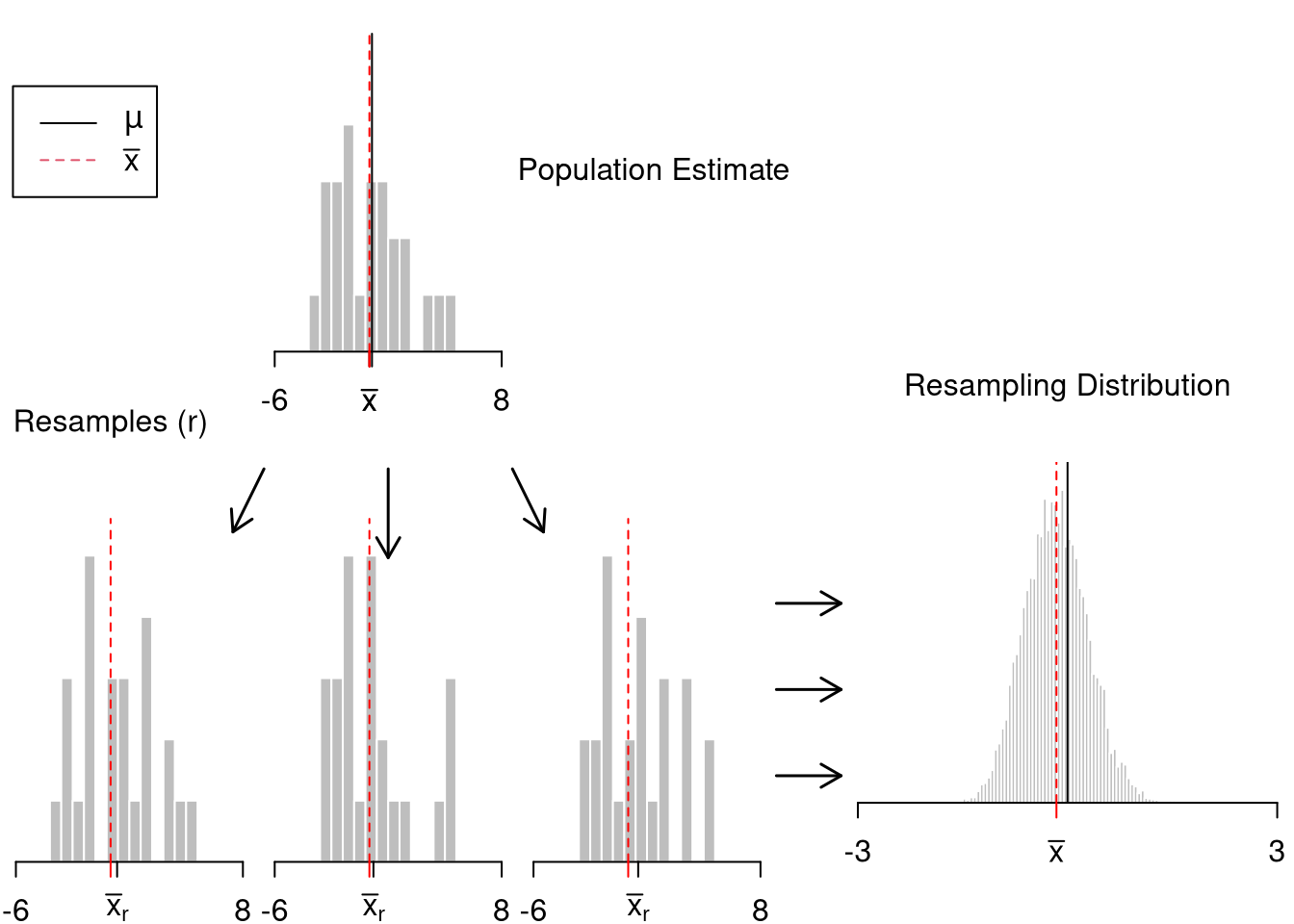
Note that we do not use the mean of the resampled statistics as a replacement for the original estimate. This is because the resampled distributions are centered at the observed statistic, not the population parameter. (The bootstrapped mean is centered at the sample mean, for example, not the population mean.) This means that we cannot use resampling to improve on \(\overline{x}\). We use resampling to estimate sampling variability.

Jackknife Distribution.

Here, we compute all “leave-one-out” estimates. Specifically, for a dataset with \(n\) observations, the jackknife uses \(n-1\) observations other than \(i\) for each unique subsample. Taking the mean, for example, we have

Code

sample_dat <- USArrests[,'Murder']
sample_mean <- mean(sample_dat)

# Jackknife Estimates
n <- length(sample_dat)
Jmeans <- sapply(1:n, function(i){
    dati <- sample_dat[-i]
    mean(dati)
})
hist(Jmeans, breaks=25, border=NA,
    main='', xlab=expression(bar(X)[-i]))
abline(v=sample_mean, col='red', lty=2)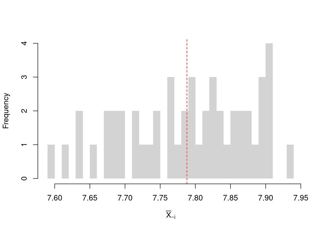

Bootstrap Distribution.

Here, we draw \(n\) observations with replacement from the original data to create a bootstrap sample and calculate a statistic. Each bootstrap sample \(b=1...B\) uses a random set of observations (denoted \(N_{b}\)) to compute a statistic. We repeat that many times, say \(B=9999\), to estimate the sampling distribution. Consider the sample mean as an example;

Code

# Bootstrap estimates
set.seed(2)
Bmeans <- sapply(1:10^4, function(i) {
    dat_b <- sample(sample_dat, replace=T) # c.f. jackknife
    mean(dat_b)
})

hist(Bmeans, breaks=25, border=NA,
    main='', xlab=expression(bar(X)[b]))
abline(v=sample_mean, col='red', lty=2)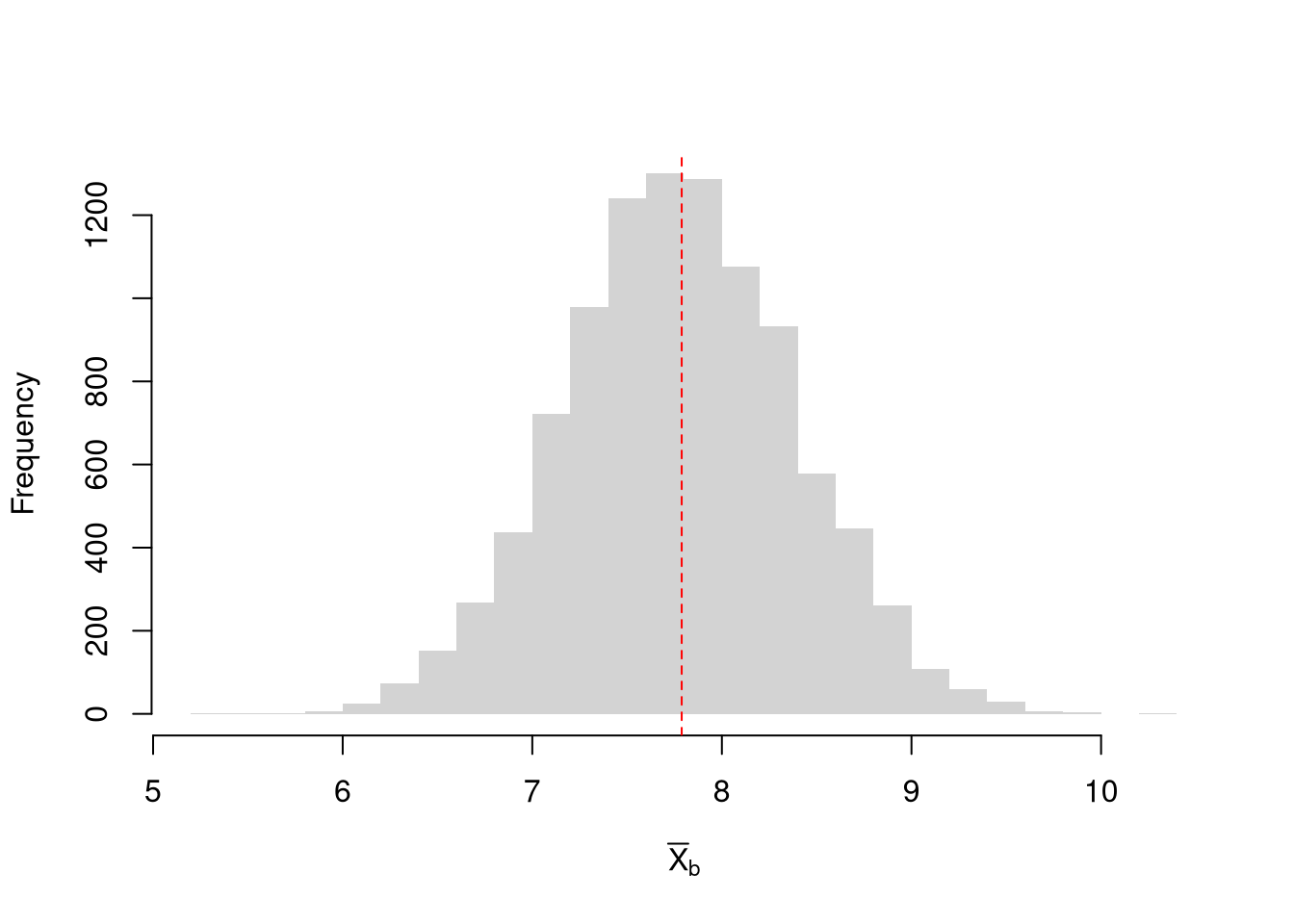

Note that both resampling methods provide imperfect estimates, and can give different numbers. Percentiles of jackknife resamples are systematically less variable than they should be. Until you know more, a conservative approach is to take the larger estimate.

Code

# Boot CI
boot_ci <- quantile(Bmeans, probs=c(.025, .975))
boot_ci
##    2.5%   97.5% 
## 6.58200 8.97005

# Jack CI
jack_ci <- quantile(Jmeans, probs=c(.025, .975))
jack_ci
##     2.5%    97.5% 
## 7.621582 7.904082

# more conservative estimate
ci_est <- boot_ci

6.3 Intervals

Using either the bootstrap or jackknife distribution for subsamples, or across multiple samples if we can get them, we can calculate

Confidence Interval: range your statistic varies across different samples.
Standard Error: variance of your statistic across different samples (square rooted).

Code

sample_means <- apply(x,1,mean)
# standard error
sd(sample_means)
## [1] 0.01679171

Note that in some cases, you can estimate the standard error to get a confidence interval.

Code

x00 <- x[1,]
# standard error
s00 <- sd(x00)/sqrt(length(x00))
ci <- mean(x00) + c(1.96, -1.96)*s00

Confidence Interval.

Compute the upper and lower quantiles of the sampling distribution.

For example, consider the sample mean. We simulate the sampling distribution of the sample mean and construct a 90% confidence interval by taking the 5th and 95th percentiles of the simulated means. This gives an empirical estimate of the interval within which the true mean is expected to lie with 90% confidence, assuming repeated sampling.

Code

# Middle 90%
mq <- quantile(sample_means, probs=c(.05,.95))
paste0('we are 90% confident that the mean is between ', 
    round(mq[1],2), ' and ', round(mq[2],2) )
## [1] "we are 90% confident that the mean is between 0.47 and 0.53"

bks <- seq(.4,.6,by=.001)
hist(sample_means, breaks=bks, border=NA,
    col=rgb(0,0,0,.25), font.main=1,
    main='Confidence Interval for the mean')
abline(v=mq)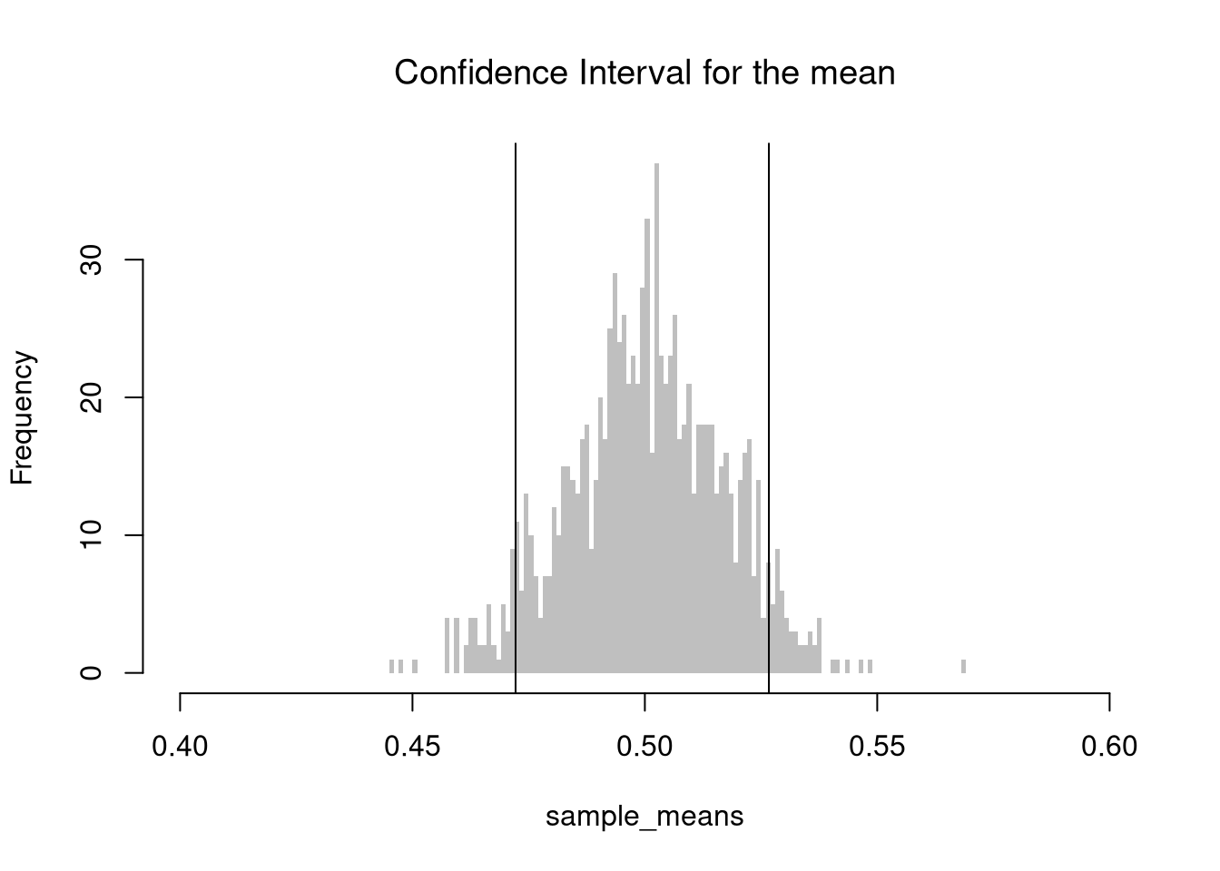

For another example, consider an extreme sample percentile. We now repeat the above process to estimate the 99th percentile for each sample, instead of the mean for each sample. We then construct a 95% confidence interval for the 99th percentile estimator, using the 2.5th and 97.5th quantiles of these estimates.

Code

## Upper Percentile
sample_quants <- apply(x,1,quantile, probs=.99)

# Middle 95% of estimates
mq <- quantile(sample_quants, probs=c(.025,.975))
paste0('we are 95% confident that the upper percentile is between ', 
    round(mq[1],2), ' and ', round(mq[2],2) )
## [1] "we are 95% confident that the upper percentile is between 0.97 and 1"

bks <- seq(.92,1,by=.001)
hist(sample_quants, breaks=bks, border=NA,
    col=rgb(0,0,0,.25), font.main=1,
    main='95% Confidence Interval for the 99% percentile')
abline(v=mq)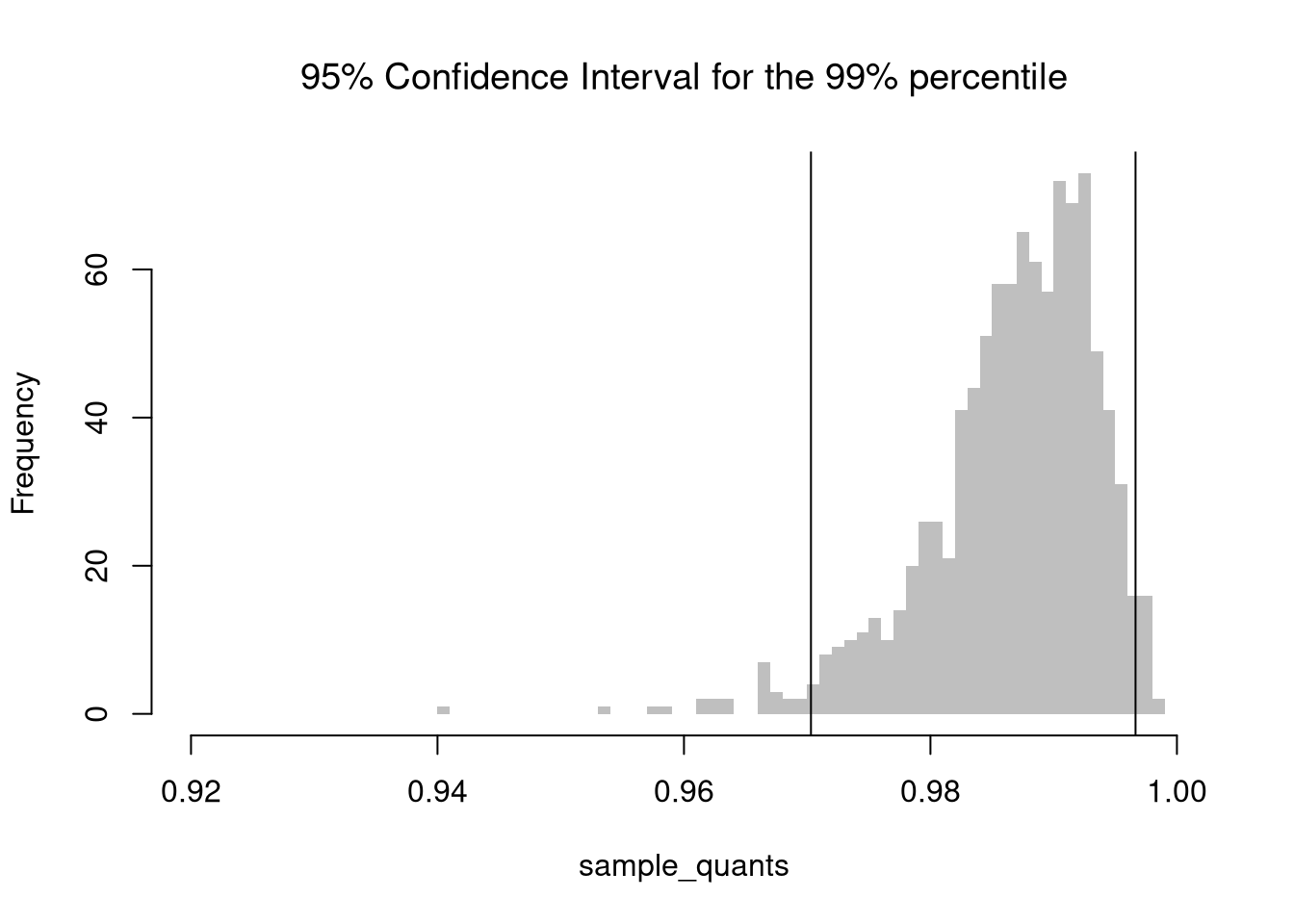

Note that \(X%\) confidence intervals do not generally cover \(X%\) of the data. Those intervals are a type of prediction interval that is covered later. See also https://online.stat.psu.edu/stat200/lesson/4/4.4/4.4.2.

Advanced Intervals.

In many cases, we want a X% interval to mean that X% of the intervals we generate will contain the true mean. E.g., in repeated sampling, 50% of constructed confidence intervals are expected to contain the true population mean.

Code

# Theoretically: [-1 sd, +1 sd] has 2/3 coverage

# Confidence Interval for each sample
xq <- apply(x,1, function(r){ #theoretical se's 
    mean(r) + c(-1,1)*sd(r)/sqrt(length(r))
})
# First 4 interval estimates
xq[,1:4]
##           [,1]      [,2]      [,3]      [,4]
## [1,] 0.4588823 0.5157968 0.4822444 0.5081667
## [2,] 0.4917643 0.5498029 0.5155981 0.5404135

# Explicit calculation
mu_true <- 0.5
# Logical vector: whether the true mean is in each CI
covered <- mu_true >= xq[1, ] & mu_true <= xq[2, ]
# Empirical coverage rate
coverage_rate <- mean(covered)
cat(sprintf("Estimated coverage probability: %.2f%%\n", 100 * coverage_rate))
## Estimated coverage probability: 67.80%

Code

# Visualize first N confidence intervals
N <- 100
plot.new()
plot.window(xlim = range(xq), ylim = c(0, N))
for (i in 1:N) {
  col_i <- if (covered[i]) rgb(0, 0, 0, 0.3) else rgb(1, 0, 0, 0.5)
  segments(xq[1, i], i, xq[2, i], i, col = col_i, lwd = 2)
}
abline(v = mu_true, col = "blue", lwd = 2)
axis(1)
title("Visualizing CI Coverage (Red = Missed)")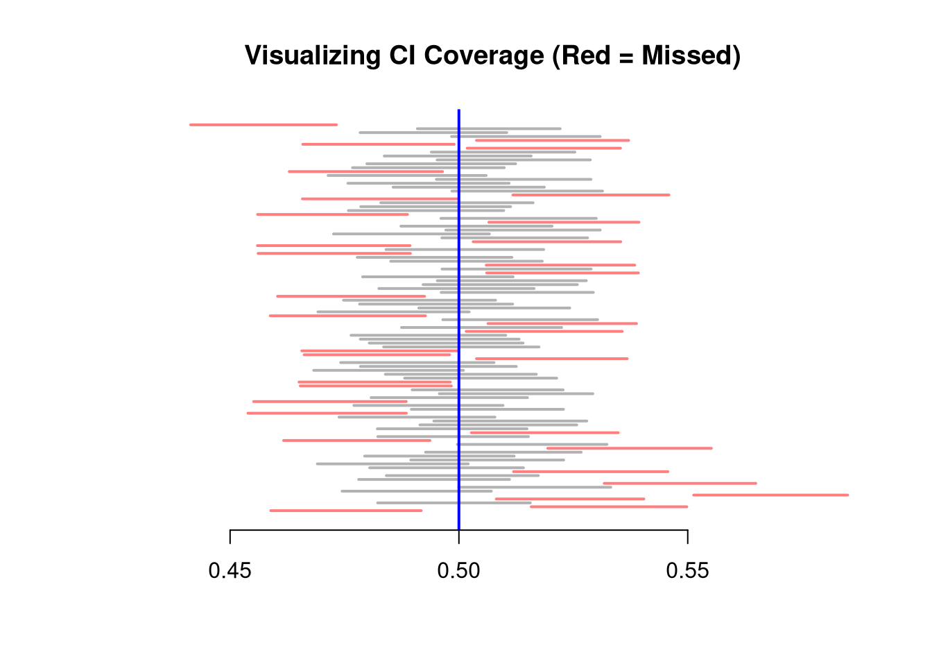

This differs from a pointwise inclusion frequency interval

Code

# Frequency each point was in an interval
bks <- seq(0,1,by=.01)
xcovr <- sapply(bks, function(b){
    bl <- b >= xq[1,]
    bu <- b <= xq[2,]
    mean( bl & bu )
})
# 50\% Coverage
c_ul <- range(bks[xcovr>=.5])
c_ul # 50% confidence interval
## [1] 0.49 0.51

plot.new()
plot.window(xlim=c(0,1), ylim=c(0,1))
polygon( c(bks, rev(bks)), c(xcovr, xcovr*0), col=grey(.5,.5), border=NA)
mtext('Frequency each value was in an interval',2, line=2.5)
axis(1)
axis(2)
abline(h=.5, lwd=2)
segments(c_ul,0,c_ul,.5, lty=2)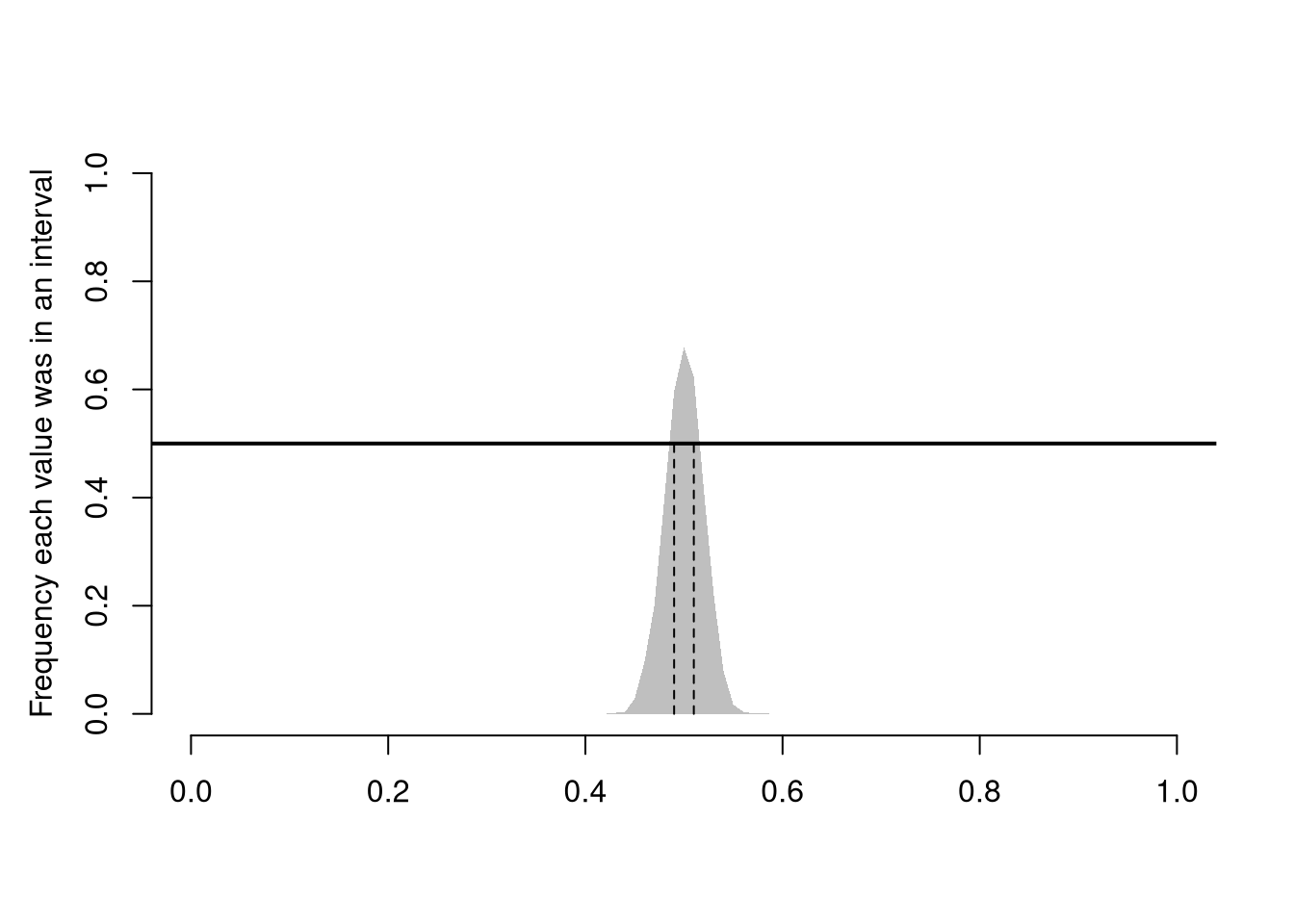

6.4 Standard Errors

Note that the standard deviation refers to variance within a single sample, and is hence different from the standard error. Nonetheless, they can both be used to estimate the variability of a statistic.

Code

boot_se <- sd(Bmeans)

sample_sd <- sd(sample_dat)
theory_se <- sample_sd/sqrt(n)

c(boot_se, theory_se)
## [1] 0.6056902 0.6159621

A famous theoretical result in statistics is that if we have independent and identical data (i.e., that each new \(X_{i}\) has the same mean \(\mu\) and same variance \(\sigma^2\) and is drawn without any dependence on the previous draws), then the standard error of the sample mean is “root N” proportional to the theoretical standard error. \[\begin{eqnarray} \mathbb{V}\left( \bar{X} \right) &=& \mathbb{V}\left( \frac{\sum_{i}^{n} X_{i}}{n} \right) = \sum_{i}^{n} \mathbb{V}\left(\frac{X_{i}}{n}\right) = \sum_{i}^{n} \frac{\sigma^2}{n^2} = \sigma^2/n\\ \mathbb{s}\left(\bar{X}\right) &=& \sqrt{\sigma^2/n} = \sigma/\sqrt{n}. \end{eqnarray}\]

Notice that each additional data point you have provides more information, which ultimately decreases the standard error of your estimates. This is why statisticians will often recommend that you to get more data. However, the improvement in the standard error increases at a diminishing rate. In economics, this is known as diminishing returns and why economists may recommend you do not get more data.

Code

Nseq <- seq(1,100, by=1) # Sample sizes
B <- 1000 # Number of draws per sample

SE <- sapply(Nseq, function(n){
    sample_statistics <- sapply(1:B, function(b){
        x <- rnorm(n) # Sample of size N
        quantile(x,probs=.4) # Statistic
    })
    sd(sample_statistics)
})

par(mfrow=c(1,2))
plot(Nseq, SE, pch=16, col=grey(0,.5),
    main='Absolute Gain', font.main=1,
    ylab='standard error', xlab='sample size')
plot(Nseq[-1], abs(diff(SE)), pch=16, col=grey(0,.5),
    main='Marginal Gain', font.main=1,
    ylab='decrease in standard error', xlab='sample size')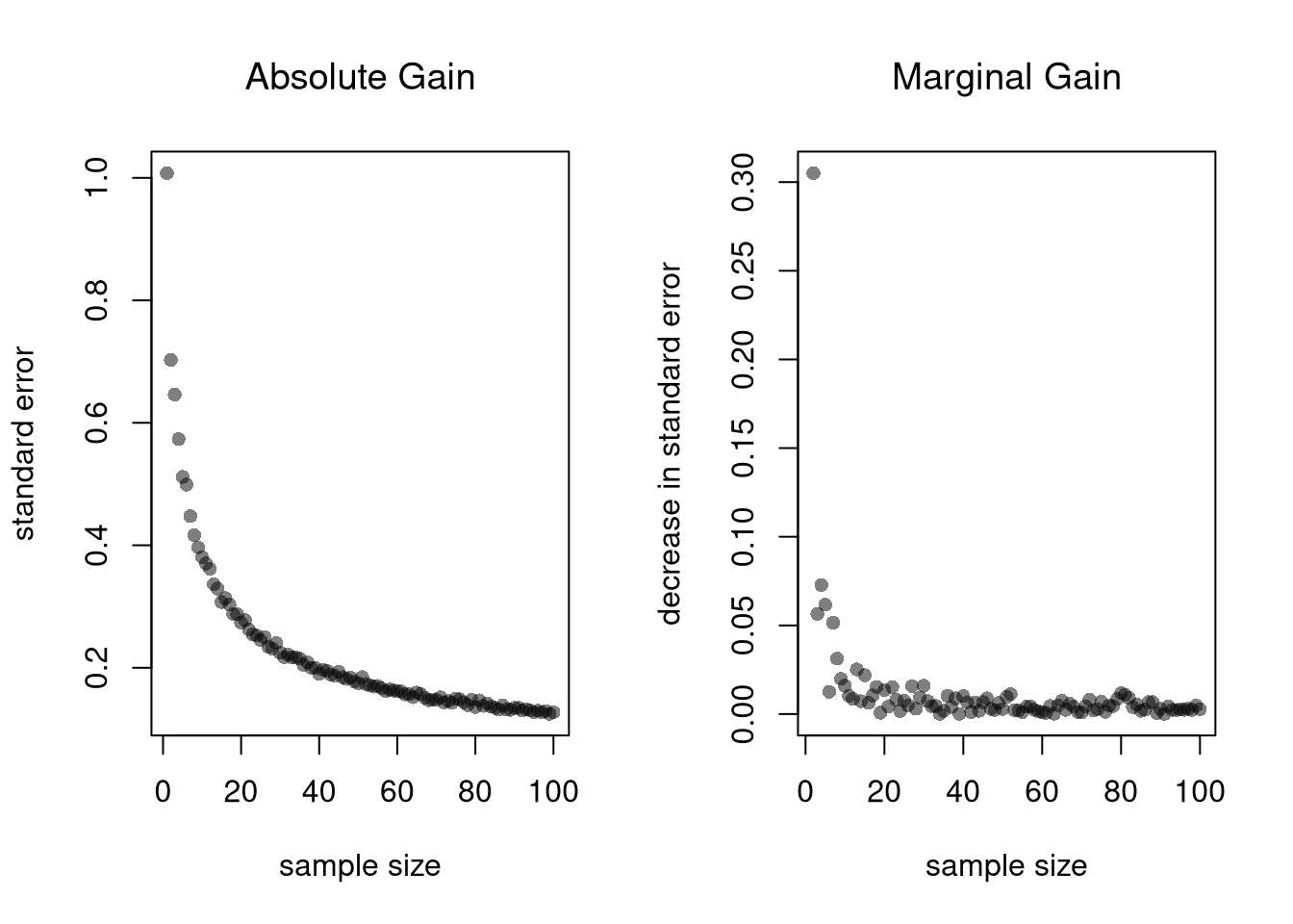

6.5 Further Reading

See

https://www.r-bloggers.com/2025/02/bootstrap-vs-standard-error-confidence-intervals/