4 Random Variables
4.1 Introduction
Previously, we computed a distribution given the data, whereas now we generate individual data points given the distribution.
Random variables are variables whose values occur according to a frequency distribution. As such, random variables have a
- sample space which refers to the set of all possible outcomes, and
- probability for each particular set of outcomes, which is the proportion that those outcomes occur in the long run.
We think of a data generating process before the data are actually observed. For example, we consider flipping a coin before knowing whether it lands on heads or tails. We denote the random variable, in this case the unflipped coin, as \(X_{i}\), and the specific values it can take as \(x\) (\(x=1\) is heads, \(x=0\) is tails) and the probability of each outcome is \(1/2\). This differs from a flipped coin that is either heads or tails, and denoted as \(\hat{X}_{i}\).
There are two basic types of sample spaces: discrete (encompassing cardinal-discrete, factor-ordered, and factor-unordered data) and continuous. This leads to two types of random variables: discrete and continuous. However, each type has many different probability distributions.
Cumulative Probability.
The most common random variables are easily accessible and can be described using the cumulative distribution function (CDF) \[\begin{eqnarray} F(x) &=& Prob(X_{i} \leq x). \end{eqnarray}\] Note that this is just like the Empirical Cumulative Distribution Function (ECDF), \(\hat{F}(x)\), except that it is now theoretically known. You can think of \(F(x)\) as the ECDF for a dataset with an infinite number of observations. Equivalently, the ECDF is an empirical version of the CDF that is applied to observed data.
Probability Rules.
After introducing different random variables, we will also cover some basic implications of their CDF. Intuitively, probabilities must sum up to one. So we can compute \(Prob(X_{i} > x) = 1- F(x)\). We also have two “in” and “out” probabilities.
The probability of \(X_{i}\leq b\) and \(X_{i}> a\) can be written in terms of falling into a range \(Prob(X_{i} \in (a,b])=Prob(a < X_{i} \leq b) = F(b) - F(a)\).
The opposite probability of \(X_{i} > b\) or \(X_{i} \leq a\) is \(Prob(X_{i} \leq a \text{ or } X_{i} > b) = F(a) + [1- F(b)]\). Notice that this opposite probability \(F(a) + [1- F(b)] =1 - [F(b) - F(a)]\), so that \(Prob(X_{i} \text{ out of } (a,b]) = 1 - Prob( X_{i} \in (a,b])\)
4.2 Discrete Random Variables
A discrete random variable can take one of several values in a set. E.g., any number in \(\{1,2,3,...\}\) or any letter in \(\{A,B,C,...\}\). Theoretical proportions are referred to as a probability mass function, which can be thought of as a proportions bar plot for an infinitely large dataset. Equivalently, the bar plot is an empirical version of the probability mass function that is applied to observed data.
In R, you can simulate random discrete data using the sample function. To do so, you must specify each outcome \(x\) and its probability \(Prob(X_{i}=x)\).
Bernoulli.
Think of a Coin Flip: Heads or Tails with equal probability. In general, a Bernoulli random variable denotes heads as the event \(x=1\) and tails as the event \(x=0\), and allows the probability of heads to vary \(p \in [0,1]\). \[\begin{eqnarray} X_{i} &\in& \{0,1\} \\ Prob(X_{i} =0) &=& 1-p \\ Prob(X_{i} =1) &=& p \\ F(x) &=& \begin{cases} 0 & x<0 \\ 1-p & x \in [0,1) \\ 1 & x\geq 1 \end{cases} \end{eqnarray}\]
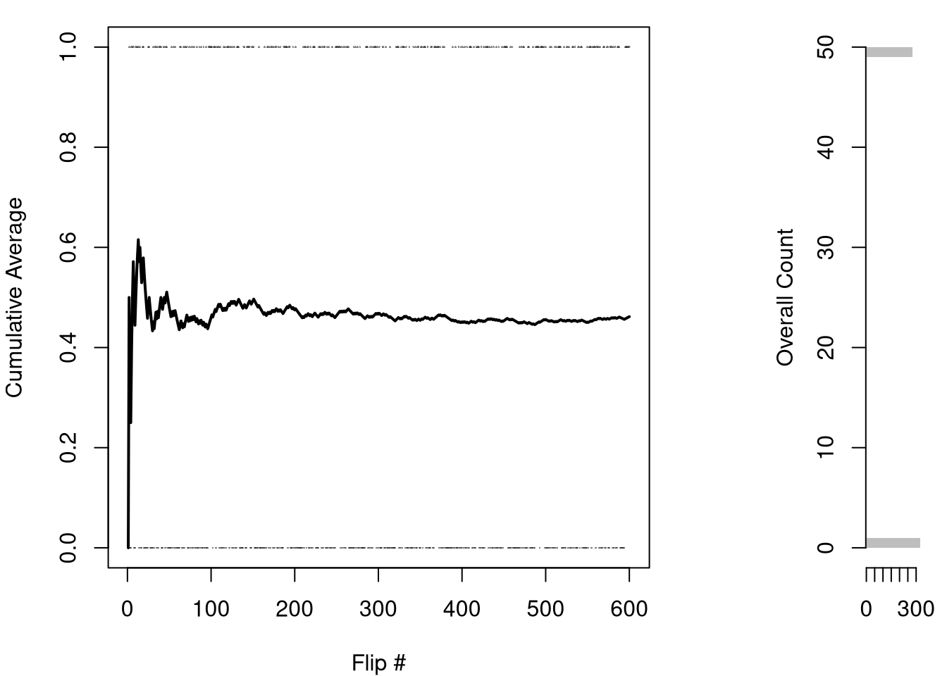
Here is an example of the Bernoulli distribution. While you might get all heads (or all tails) in the first few coin flips, the ratios level out to their theoretical values after many flips.
Code
x <- c(0, 1)
x_probs <- c(3/4, 1/4)

sample(x, 1, prob=x_probs, replace=T) # 1 Flip
## [1] 0
sample(x, 4, prob=x_probs, replace=T) # 4 Flips
## [1] 1 0 0 0
X0 <- sample(x, 400, prob=x_probs, replace=T)

# Plot proportions
proportions <- table(X0)/length(X0)
plot(proportions,
    col=grey(0, 0.5),
    xlab='Flip Outcome',
    ylab='Proportion',
    main=NA)
points(c(0, 1), c(.75, .25), pch=16, col=rgb(0, 0, 1, .8)) # Theoretical values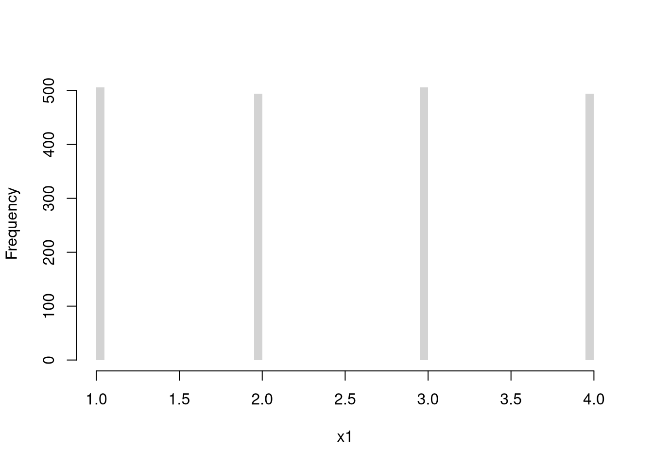
Code
# Plot CDF
plot( ecdf(X0), col=grey(0, .5),
    pch=16, main=NA) #Empirical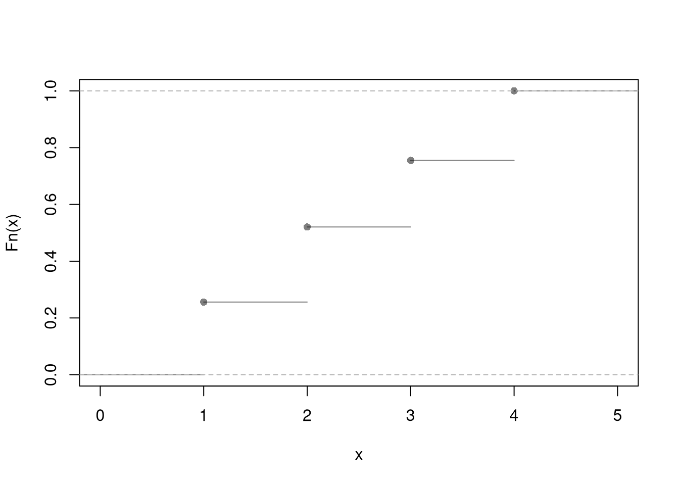
Code
#points(c(0, 1), c(.75, 1), pch=16, col='blue') # TheoreticalDiscrete Uniform.
Discrete numbers with equal probability, such as a die with \(K\) sides. \[\begin{eqnarray} X_{i} &\in& \{1,...K\} \\ Prob(X_{i} =1) &=& Prob(X_{i} =2) = ... = 1/K\\ F(x) &=& \begin{cases} 0 & x<1 \\ 1/K & x \in [1,2) \\ 2/K & x \in [2,3) \\ \vdots & \\ 1 & x\geq K \end{cases} \end{eqnarray}\]
Code
x <- c(1, 2, 3, 4)
x_probs <- c(1/4, 1/4, 1/4, 1/4)
# sample(x, 1, prob=x_probs, replace=T) # 1 roll
X1 <- sample(x, 2000, prob=x_probs, replace=T) # 2000 rolls

# Plot Long run proportions
proportions <- table(X1)/length(X1)
plot(proportions, col=grey(0, .5),
    xlab='Outcome', ylab='Proportion', main=NA)
points(x, x_probs, pch=16, col=rgb(0, 0, 1, .8)) # Theoretical values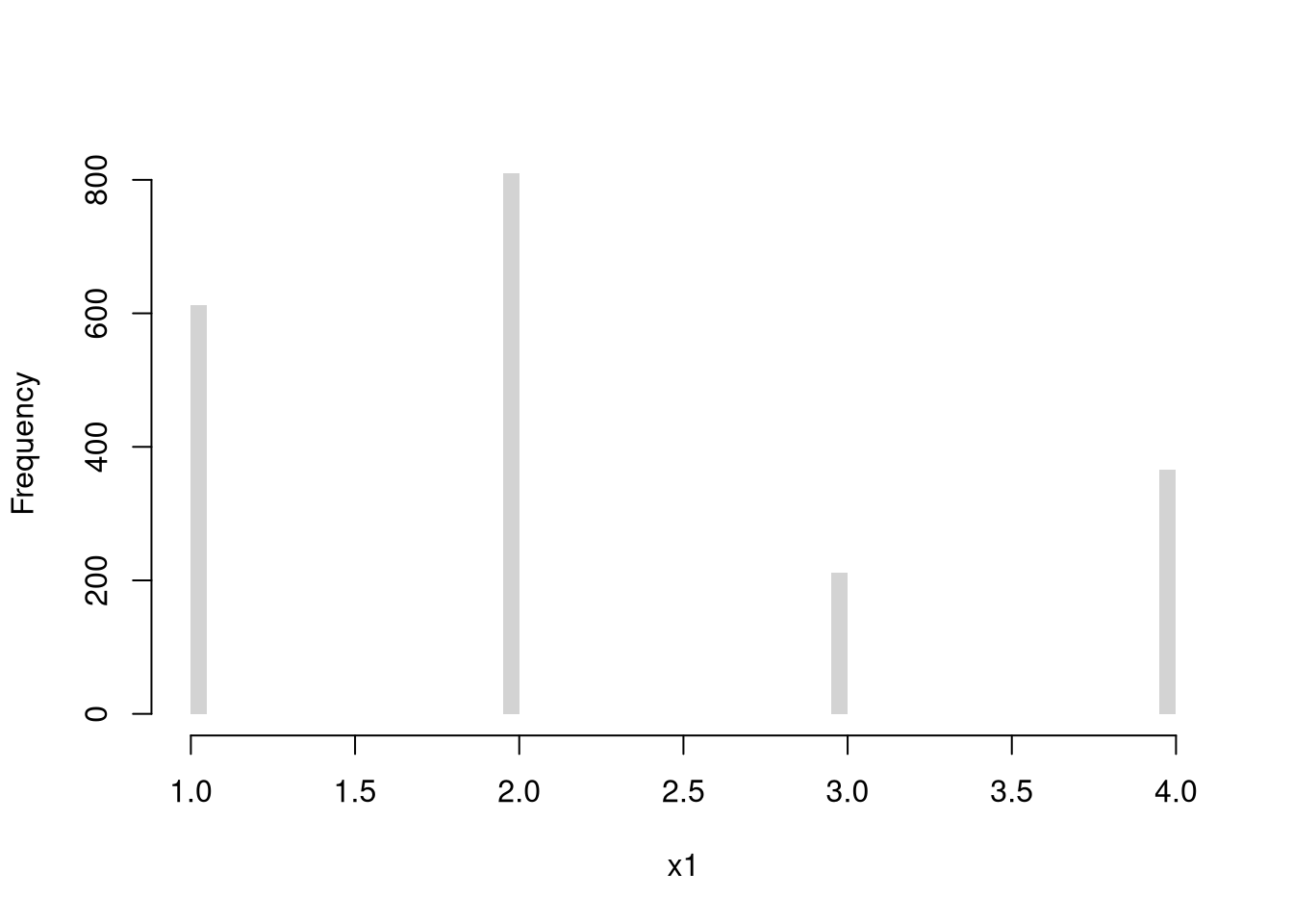
Code
# Hist w/ Theoretical Counts
# hist(X1, breaks=50, border=NA, main=NA, ylab='Count')
# points(x, x_probs*length(X1), pch='-')

# Alternative Plot
plot( ecdf(X1), pch=16, col=grey(0, .5), main=NA)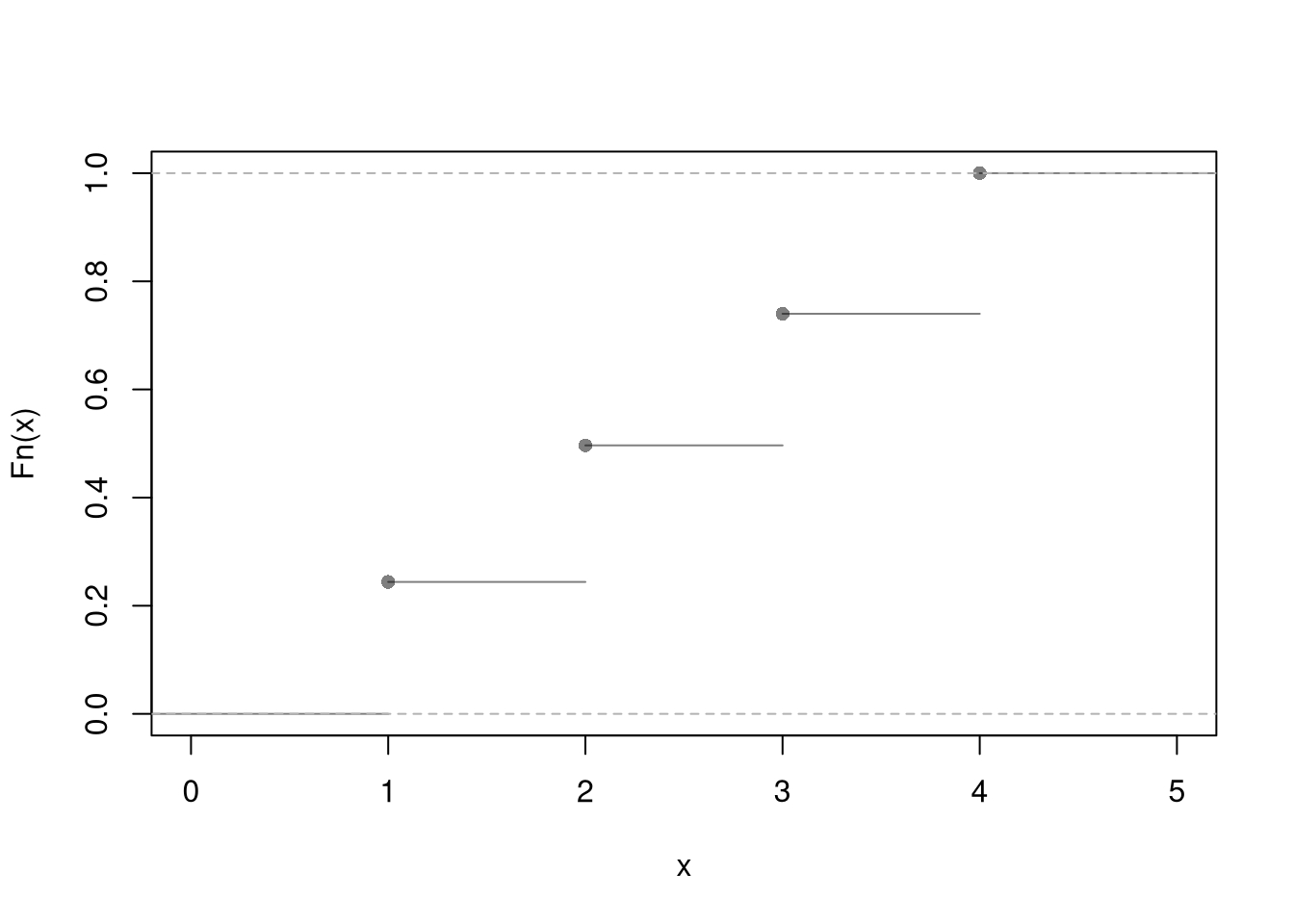
Code
# Alternative Plot 2
#props <- table(X1)
#barplot(props, ylim = c(0, 0.35), ylab = 'Proportion', xlab = 'Value')
#abline(h = 1/4, lty = 2)
Note that the Discrete Uniform distribution generalizes to arbitrary sets, such as \(\{0.0, 0.25, 0.5, 0.75, 1.0\}\) instead of \(\{1,2,3,4,5\}\). We will not exploit the generalization in this class.
Multinoulli.
Numbers \(1,...K\) with unequal probabilities. \[\begin{eqnarray} X_{i} &\in& \{1,...K\} \\ Prob(X_{i} =1) &=& p_{1} \\ Prob(X_{i} =2) &=& p_{2} \\ &\vdots& \\ p_{1} + p_{2} + ... &=& 1\\ F(x) &=& \begin{cases} 0 & x<1 \\ p_{1} & x \in [1,2) \\ p_{1} + p_{2} & x \in [2,3) \\ \vdots & \\ 1 & x\geq K \end{cases} \end{eqnarray}\]
Here is an empirical example with three outcomes
Code
x <- c(1, 2, 3)
x_probs <- c(3/10, 1/10, 6/10)
sum(x_probs)
## [1] 1
X2 <- sample(x, 2000, prob=x_probs, replace=T) # sample of 2000

# Plot Long run proportions
proportions <- table(X2)/length(X2)
plot(proportions, col=grey(0, .5), ylim=c(0, 0.7),
    xlab='Outcome', ylab='Proportion', main=NA)
points(seq(x), x_probs, pch=16, col=rgb(0, 0, 1, .8)) # Theoretical values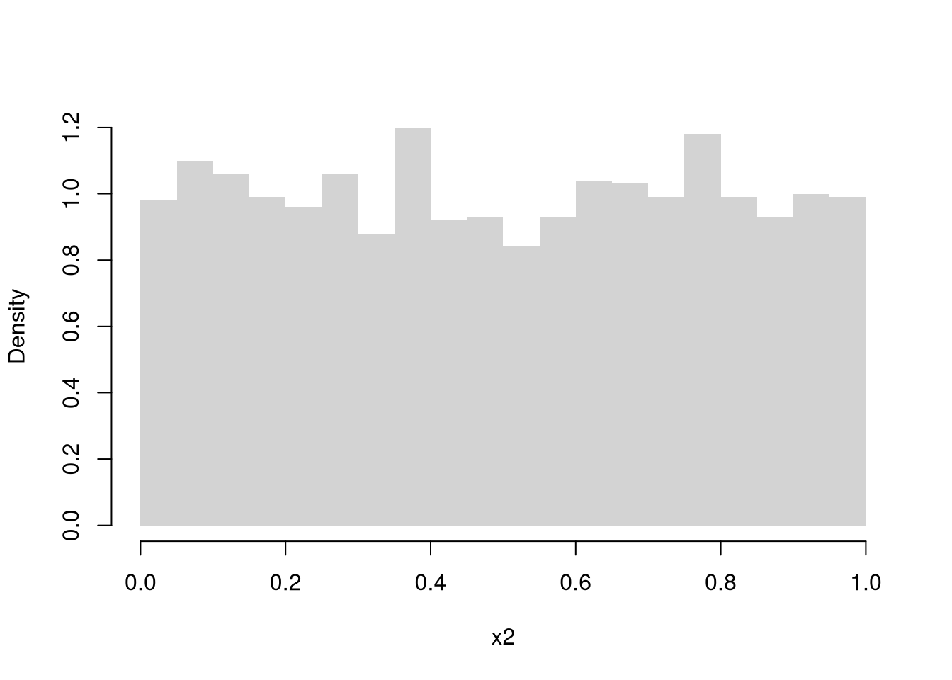
Code
# Histogram version
# X2_alt <- X1
# X2_alt[X2_alt=='A'] <- 1
#X2_alt[X2_alt=='B'] <- 2
#X2_alt[X2_alt=='C'] <- 3
#X2_alt <- as.numeric(X1_alt)
#hist(X2_alt, breaks=50, border=NA,
#    main=NA, ylab='Count')
#points(x, x_probs*length(X2_alt), pch=16) ## Theoretical Counts

# Alternative Plot
# plot( ecdf(X2), pch=16, col=grey(0, .5), main=NA)
We can also replace numbers with letters \((A,...Z)\) or names \((John, Jamie, ...)\) although we must be careful with the CDF when there is no longer a natural ordering. When the outcomes are not cardinal data, the Multinoulli random variable is typically referred to as a Categorical random variable. The CDF \(F(x)=Prob(X_{i} \leq x)\) requires an ordering on the outcomes, and with labels like “my car dies” and “it rains next Tuesday”, you do not have any inherent order and the CDF is an arbitrary artifact.
4.3 Continuous Random Variables
A continuous random variable can take one value out of an uncountably infinite number. E.g., any number between \(0\) and \(1\) with any number of decimal points. With a continuous random variable, the probability of any individual point is zero, so we describe these variables with the cumulative distribution function (CDF), \(F\), or the probability density function (PDF), \(f\). Just as \(F\) can be thought of as the ECDF, \(\hat{F}\), with an infinite amount of data, \(f\) can be thought of as a histogram, \(\hat{f}\), with an infinite amount of data. Equivalently, the histogram is an empirical version of the PDF that is applied to observed data.
Often, the PDF helps you intuitively understand a random variable whereas the CDF helps you calculate numerical values. This is because probabilities are depicted as areas in the PDF and the CDF accumulates those areas: \(F(x)\) equals the area under the PDF from \(-\infty\) to \(x\). For example, \(Prob(X_{i} \leq 1)\) is depicted by the PDF as the area under \(f(x)\) from the lowest possible value until \(x=1\), which is numerically calculated simply as \(F(1)\).
In R, you work with continuous distributions these using functions
dXXXdensity, \(f(x)\) for particular values \(x\)pXXXdistribution, \(F(x)\) for particular values \(x\)rXXXgenerate random variables according to the distribution
where XXX is the distribution name (unif, exp, norm)
Continuous Uniform.
Any number on a unit interval allowing for any number of decimal points, with every interval of the same size having the same probability. \[\begin{eqnarray} X_{i} &\in& [0,1] \\ f(x) &=& \begin{cases} 1 & x \in [0,1] \\ 0 & \text{Otherwise} \end{cases}\\ F(x) &=& \begin{cases} 0 & x < 0 \\ x & x \in [0,1] \\ 1 & x > 1. \end{cases} \end{eqnarray}\]
Code
runif(3) # 3 draws
## [1] 0.8154670 0.4468603 0.7531652

# Empirical Density
X3 <- runif(2000)
hist(X3, breaks=20, border=NA, main=NA, freq=F)
# Theoretical Density
x <- seq(-0.1, 1.1, by=.001)
fx <- dunif(x)
lines(x, fx, col=rgb(0, 0, 1, .8))
Code
# CDF example 1
P_low <- punif(0.25)
P_low
## [1] 0.25
# Uncomment to show via PDF
# x_low <- seq(0, 0.25, by=.001)
# fx_low <- dunif(x_low)
# polygon( c(x_low, rev(x_low)), c(fx_low, fx_low*0),
#    col=rgb(0, 0, 1, .25), border=NA)

# CDF example 2
P_high <- 1-punif(0.25)
P_high
## [1] 0.75
# Uncomment to show via PDF
# x_high <- seq(0.25, 1, by=.001)
# fx_high <- dunif(x_high)
# polygon( c(x_high, rev(x_high)), c(fx_high, fx_high*0),
#    col=rgb(0, 0, 1, .25), border=NA)

# CDF example 3
P_mid <- punif(0.75) - punif(0.25)
P_mid
## [1] 0.5
# Uncomment to show via PDF
# x_mid <-  seq(0.25, 0.75, by=.001)
# fx_mid <- dunif(x_mid)
# polygon( c(x_mid, rev(x_mid)), c(fx_mid, fx_mid*0),
#    col=rgb(0, 0, 1, .25), border=NA)
Note that the Continuous Uniform distribution generalizes to an arbitrary interval, \(X_{i} \in [a,b]\). In this case, \(f(x)=1/[b-a]\) if \(x \in [a,b]\) and \(F(x)=[x-a]/[b-a]\) if \(x \in [a,b]\).
NoteMust Know
Suppose \(X_{i}\) is a random variable continuously distributed over \(a=-2\) and \(b=2\). What is the probability of a value smaller than \(0.25\)? First use the computer to suggest an answer: simulate \(1000\) draws and then make a histogram and an ECDF. Then find the answer mathematically using the CDF. Finally, verify the answer is intuitively correct in a figure of the PDF. You should draw by hand both the CDF and the PDF with correct axes labels and marking clearly the probability of a value smaller than \(0.25\).
Code
# Simulation
X <- runif(1000, -2, 2)
# ...

# Draw by computer the CDF, F(x)
x <- seq(-3, 3, by=0.005)
Fx <- punif(x, -2, 2)
plot(x, Fx, type='l', col=rgb(0, 0, 1, .8))
# Answer
Fstar <- punif(0.25, -2, 2)
# Visualize Answer
segments(0.25, 0, 0.25, Fstar,
    col=rgb(0, 0, 1, 0.25))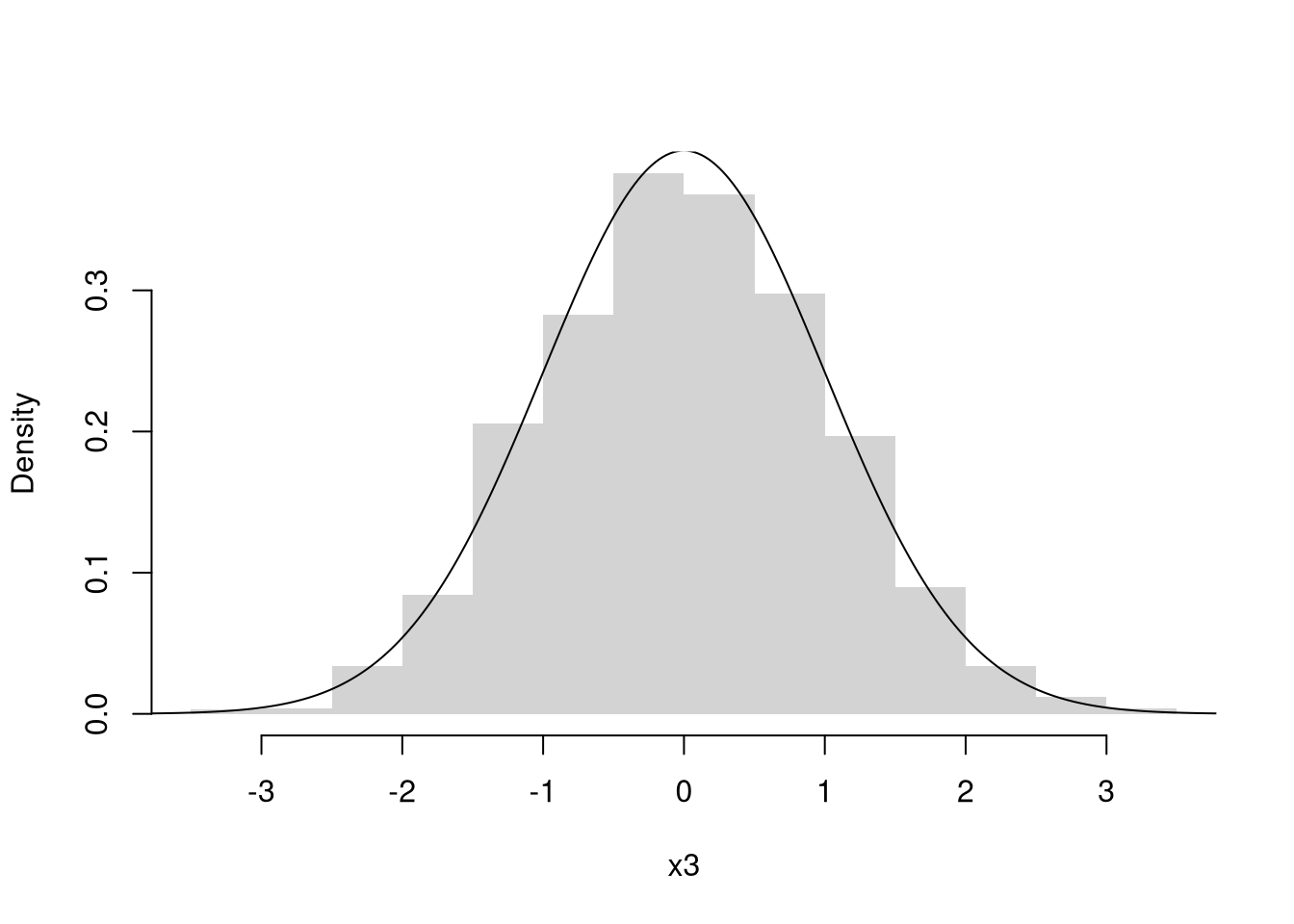
Code
# Draw by computer the PDF, f(x)
fx <- dunif(x, -2, 2)
plot(x, fx, type='l', col=rgb(0, 0, 1, .8))
# Visualize Answer
fstar <- dunif(0.25, -2, 2)
polygon(
    c(-2, 0.25, 0.25, -2),
    c(0, 0, fstar, fstar),
    col=rgb(0, 0, 1, 0.25), border=NA)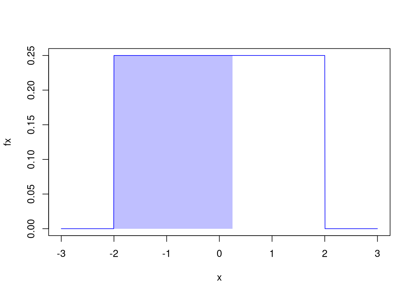
Exponential.
The sample space is any positive number.2 An Exponential random variable has a single parameter, \(\lambda>0\), that governs its shape \[\begin{eqnarray} X_{i} &\in& [0,\infty) \\ f(x) &=& \lambda exp\left\{ -\lambda x \right\} \\ F(x) &=& \begin{cases} 0 & x < 0 \\ 1- exp\left\{ -\lambda x \right\} & x \geq 0. \end{cases} \end{eqnarray}\]
Code
rexp(3) # 3 draws
## [1] 0.5874910 0.6506402 0.5505593

X5 <- rexp(2000)
hist(X5, breaks=20,
    border=NA, main=NA,
    freq=F, ylim=c(0, 1), xlim=c(0, 10))

x <- seq(0, 10, by=.1)
fx <- dexp(x)
lines(x, fx, col=rgb(0, 0, 1, .8))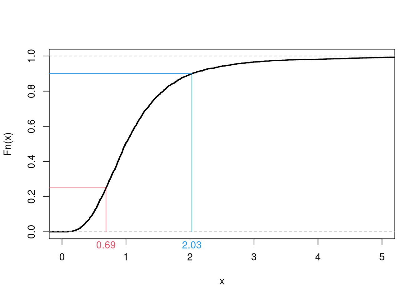
TipTest Yourself
Note that there is a discrete version of the exponential, called the geometric distribution.
Code
Y <- rexp(5000, rate=.2)

X <- rgeom(5000, 1-exp(-.2))

par(mfrow=c(1, 2))
bks <- seq(0, 50, by=0.25)
hist(X, breaks=bks, freq=F, border=NA, main=NA, xlab='x')
title('Geometric', font.main=1)
hist(floor(Y), breaks=bks, freq=F, border=NA, main=NA, xlab='x')
title('Exponential (floored)', font.main=1)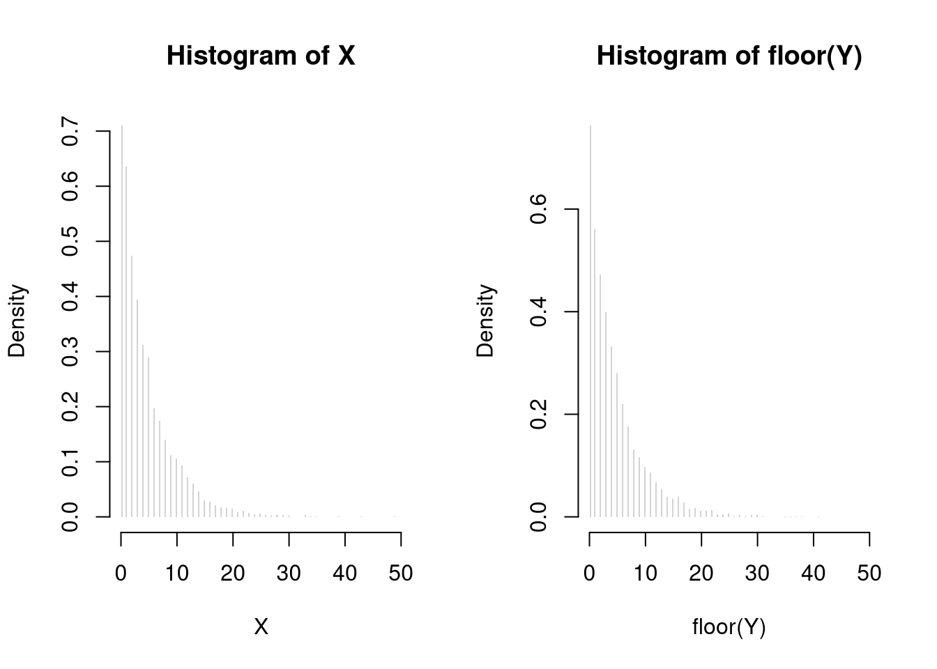
Normal (Gaussian).
This distribution is for any number on the real line, with bell shaped probabilities. The Normal distribution is mathematically complex and sometimes called the Gaussian distribution. We call it “Normal” because we will encounter it again and again and again. The probability density function \(f\) has two parameters \(\mu \in (-\infty,\infty)\) and \(\sigma > 0\). \[\begin{eqnarray} X_{i} &\in& (-\infty,\infty) \\ f(x) &=& \frac{1}{\sqrt{2\pi \sigma^2}} exp\left\{ \frac{-(x-\mu)^2}{2\sigma^2} \right\} \end{eqnarray}\]
Code
rnorm(3) # 3 draws
## [1] -1.6699733 -0.9575285 -0.9597139

X6 <- rnorm(2000)
hist(X6, breaks=20,
    border=NA, main=NA,
    freq=F, ylim=c(0, .4), xlim=c(-4, 4))

x <- seq(-10, 10, by=.025)
fx <- dnorm(x)
lines(x, fx, col=rgb(0, 0, 1, .8))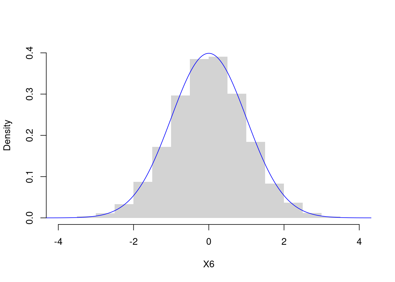
Even thought the distribution function is complex, we can compute CDF values using the computer.
Code
pnorm( c(-1.645, 1.645) ) # 10%
## [1] 0.04998491 0.95001509
pnorm( c(-2.576, 2.576) ) #  1%
## [1] 0.004997532 0.995002468
NoteMust Know
Suppose \(X_{i}\) is a random variable with a normal distribution with \(\mu=0\) and \(\sigma=1\). Intuitively depict \(Prob(X_{i} \in [0.2, 0.8])\) by drawing an area under the density function. Numerically estimate that same probability using the CDF.
Code
plot( ecdf(X6), main=NA) # Empirical

x <- seq(-4, 4, by=.01) # Theoretical
Fx <- pnorm(x, 0, 1)
lines(x, Fx, col=rgb(0, 0, 1, .8))

# Middle Interval Example
F2 <- pnorm(0.2, 0, 1)
F8 <- pnorm(0.8, 0, 1)
F_2_8 <- F8 - F2
F_2_8
## [1] 0.2088849

# Visualize
title('Middle between 0.2 and 0.8', font.main=1)
segments( 0.2, F2, -5, F2, col=rgb(1, 0, 0, .8))
segments( 0.8, F8, -5, F8, col=rgb(1, 0, 0, .8))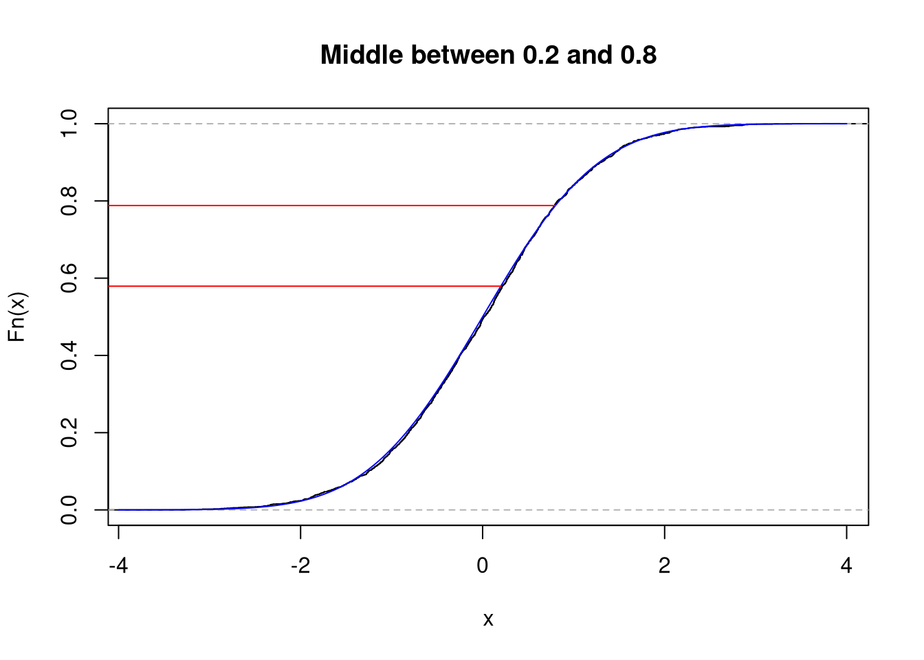
NoteMust Know
Suppose that your health status is a normally distributed random variable with \(\mu=2\) and \(\sigma=3\). If we randomly sample one person, what is the probability there health status is higher than \(4\)?
Code
# Start with a simulation of 1000 people to build intuition
X <- rnorm(1000, 2, 3)
hist(X, freq=F, border=NA, main=NA)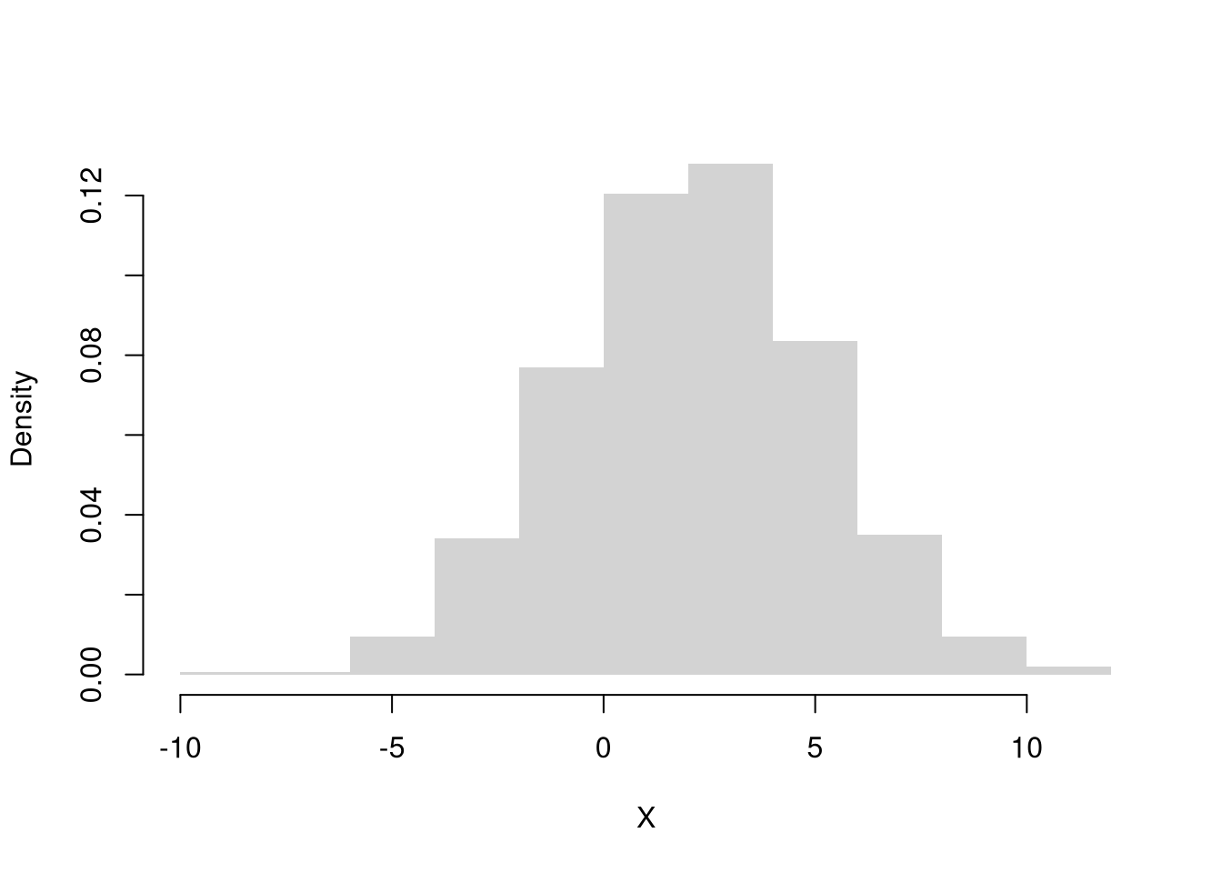
Code
sum(X>4)/1000
## [1] 0.237

# Do an exact calculation
1-pnorm(4, 2, 3)
## [1] 0.2524925
TipTest Yourself
Draw the Middle \(90\%\) of a normal distribution
Code
# PDF
x <- seq(-10, 10, by=.025)
fx <- dnorm(x)
plot(x, fx,
    col=rgb(0, 0, 1, .8), type='l',
    ylab='Theoretical Density: f(x)',
    main=NA)
title('Middle 90%', font.main=1)
# Show Middle 90%
x_90 <- seq(-1.645, 1.645, by=.025)
fx_90 <- dnorm(x_90)
polygon( c(x_90, rev(x_90)), c(fx_90, fx_90*0),
    col=rgb(0, 0, 1, .25), border=NA)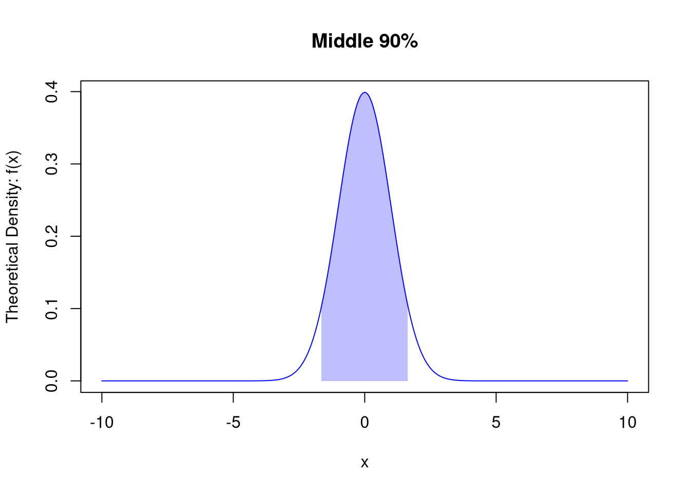
Code
pnorm(1.645)-pnorm(-1.645)
## [1] 0.90003024.4 Exercises
A Multinoulli random variable has outcomes \(\{1,2,3,4\}\) with probabilities \(\{0.1, 0.3, 0.4, 0.2\}\). Using the CDF, compute \(Prob(X_{i} \leq 2)\), \(Prob(X_{i} > 3)\), and \(Prob(1 < X_{i} \leq 3)\). Show your work.
Suppose \(X_{i}\) is normally distributed with \(\mu=10\) and \(\sigma=4\). Using
pnorm, compute the probability that \(X_{i}\) falls between \(6\) and \(14\). Then compute the probability that \(X_{i}\) is more than two standard deviations away from the mean, i.e., \(Prob(X_{i} < 2 \text{ or } X_{i} > 18)\).In R, generate \(2000\) draws from an exponential distribution with \(\lambda=0.5\) using
rexp(2000, rate=0.5). Plot a histogram withfreq=Fand overlay the theoretical density usinglinesanddexp. Then usepexpto compute the exact probability that a draw exceeds \(4\).
Further Reading.
Many random variables are related to each other. Also note that numbers randomly generated on your computer cannot be truly random, they are “pseudorandom.”
- https://en.wikipedia.org/wiki/Relationships_among_probability_distributions – Overview of how common distributions (Normal, Chi-squared, Exponential, etc.) connect to each other.
- https://www.math.wm.edu/~leemis/chart/UDR/UDR.html – Interactive chart showing transformations and limiting relationships among univariate distributions.
- https://learningstatisticswithr.com/book/probability.html – Introduction to probability distributions with worked R examples.
This is the general formula using CDFs, and you can verify it works in this instance by directly adding the probability of each 2 or 3 event: \(Prob(X_{i} = 2) + Prob(X_{i} = 3) = 1/4 + 1/4 = 2/4\).↩︎
In other classes, you may further distinguish types of random variables based on whether their maximum value is theoretically finite or infinite.↩︎