5  Statistics

---

We often summarize distributions with statistics: functions of data. The most basic way to do this is with summary, whose values can all be calculated individually.

# A random sample (real data)
X <- USArrests[,'Murder']
summary(X)
##    Min. 1st Qu.  Median    Mean 3rd Qu.    Max. 
##   0.800   4.075   7.250   7.788  11.250  17.400

# A random sample (computer simulation)
X <-  runif(1000)
summary(X)
##      Min.   1st Qu.    Median      Mean   3rd Qu.      Max. 
## 0.0000354 0.2467502 0.5023975 0.5055355 0.7582381 0.9973361

# Another random sample (computer simulation)
X <- rnorm(1000) 
summary(X)
##     Min.  1st Qu.   Median     Mean  3rd Qu.     Max. 
## -3.16047 -0.57230  0.03345  0.05981  0.74240  2.91294

Together, the mean and variance statistics summarize the central tendency and dispersion of a distribution. In some special cases, such as with the normal distribution, they completely describe the distribution. Other distributions are better described with other statistics, either as an alternative or in addition to the mean and variance. After discussing those other statistics, we will return to the two most basic statistics in theoretical detail.

5.1 Mean and Variance

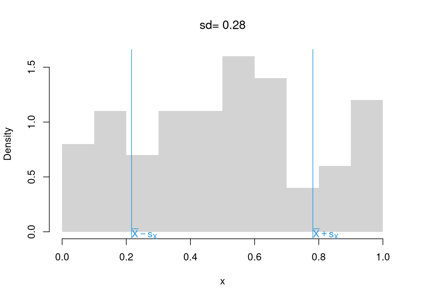
The mean and variance are the two most basic statistics that summarize the center and how spread apart the values are. As before, we represent data as vector \(\hat{X}=(\hat{X}_{1}, \hat{X}_{2}, ....\hat{X}_{n})\), where there are \(n\) observations and \(\hat{X}_{i}\) is the value of the \(i\)th one.

Mean.

Perhaps the most common statistic is the mean, which is the [sum of all values] divided by [number of values]; \[\begin{eqnarray} \hat{M} &=& \frac{\sum_{i=1}^{n}\hat{X}_{i}}{n}, \end{eqnarray}\] where \(\hat{X}_{i}\) denotes the value of the \(i\)th observation.

Note

For example, a dataset of \(\{1,4,10\}\) has a mean of \([1+4+10]/3=5\).

X <- c(1,4,10)
sum(X)/length(X)
## [1] 5
mean(X)
## [1] 5

# compute the mean of a random sample
X1 <- USArrests[,'Murder']
X1_mean <- mean(X1)
X1_mean
## [1] 7.788

# visualize on a histogram
hist(X1, border=NA, main=NA)
abline(v=X1_mean, col=2, lwd=2)
title(paste0('mean= ', round(X1_mean,2)), font.main=1)

Variance.

Perhaps the second most common statistic is the variance: the average squared deviation from the mean \[\begin{eqnarray} \hat{V} &=&\frac{\sum_{i=1}^{n} [\hat{X}_{i} - \hat{M}]^2}{n}. \end{eqnarray}\] The standard deviation is simply \(\hat{S} = \sqrt{\hat{V} }\), which can be interpreted as the average distance from the mean.

Note

For example, a dataset of \(\{1,4,10\}\) has a mean of \([1+4+10]/3=5\). The variance is \([(1-5)^2+(4-5)^2+(10-5)^2]/3=14\) and the standard deviation is \(\sqrt{14}\).

X <- c(1,4,10)
X_mean <- mean(X)
X_var <- mean( (X - X_mean)^2 )
sqrt(X_var)
## [1] 3.741657

X1_s <- sd(X1) # sqrt(var(X))
hist(X1, border=NA, main=NA, freq=F)
X1_s_lh <- c(X1_mean - X1_s,  X1_mean + X1_s)
abline(v=X1_s_lh, col=4)
text(X1_s_lh, -.02,
    c( expression(bar(X)-s[X]), expression(bar(X)+s[X])),
    col=4, adj=0)
title(paste0('sd= ', round(X1_s,2)), font.main=1)

Tip

Note that a “corrected version” is used by R and many statisticians: \(\hat{V}' =\frac{\sum_{i=1}^{n} [\hat{X}_{i} - \hat{M}]^2}{n-1}\) and \(\hat{S}' = \sqrt{\hat{V}'}\). In this class, we use the “unocorrect version” as defined previously. There is hardly any difference when \(n\) is large: e.g., \(\frac{1}{n}\approx \frac{1}{n-1}\) for \(n=100,000\).

X <- c(1,4,10)

X_mean <- mean(X)
X_var <- mean( (X - X_mean)^2 )
X_var
## [1] 14

# Corrected Version
n <- length(X)  
X_var2 <- sum( (X - X_mean)^2 )/(n-1)
X_var2
## [1] 21

var(X) # R-Version
## [1] 21

5.2 Other Center/Spread Statistics

A general rule of applied statistics is that there are multiple ways to measure something. Mean and Variance are measurements of Center and Spread, but there are others that have different theoretical properties and may be better suited for your dataset.

Medians and Absolute Deviations.

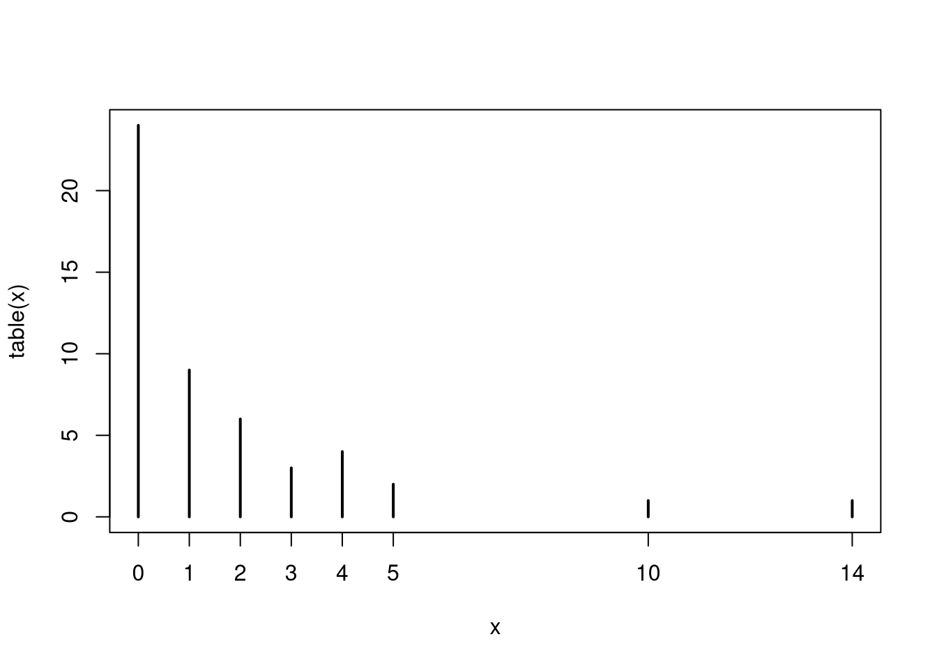
We can use the Median as a “robust alternative” to means that is especially useful for data with asymmetric distributions and extreme values. Recall that the \(q\)th quantile is the value where \(q\) percent of the data are below and (\(1-q\)) percent are above. The median (\(q=.5\)) is the point where half of the data is lower values and the other half is higher. This means that median is not sensitive to extreme values (whereas the mean is).

X <- rexp(50, 0.4)
X
##  [1] 0.2377477 0.3370880 0.5623038 3.9325224 0.4626530 3.4668011 0.2253733
##  [8] 1.0816935 2.7990144 0.1151907 3.9953716 7.7553737 2.0468143 2.3133158
## [15] 1.2667414 1.3810045 0.6626726 2.0469753 1.1354273 1.9218345 1.9700329
## [22] 5.1300768 0.4139846 0.6464575 3.8448722 7.4550862 0.7383498 4.7345013
## [29] 7.3620641 1.9860088 0.7605270 2.5145625 2.4814096 1.1273328 0.7472673
## [36] 3.5585016 1.0787746 2.6878249 0.2509548 0.1953127 0.7961368 2.0053247
## [43] 1.5521530 1.2723019 6.6406595 0.4399545 1.4130783 5.0119997 3.6853065
## [50] 0.7880215
hist(X, freq=F, breaks=seq(0,16),
    border=NA, main='')

# For discrete numbers
# X <- rgeom(50, .4)
#proportions <- table(X)/length(X)
#plot(proportions, ylab='proportion')

Note

Examine robustness to an extreme value

X_extreme <- c(X, 1000) # add one extreme value
#par(mfrow=c(1,2)) # visualize side-by-side
#hist(X)
#hist(X_extreme)


# Which measures of central tendency are robust
# to a single extreme value?
mean(X)
## [1] 2.220695
mean( X_extreme )
## [1] 21.785

quantile(X, prob=0.5)
##      50% 
## 1.482616
quantile(X_extreme, prob=0.5)
##      50% 
## 1.552153

We can also use the Interquartile Range or Median Absolute Deviation as an alternative to variance. The difference between the first and third quartiles (\(q=.25\) and \(q=.75\)) measure is range of the middle \(50%\) of the data, which is how the boxplot measures “spread”. The median absolute deviation is another statistic that also measures “spread”. \[\begin{eqnarray} \tilde{M} &=& Med( \hat{X}_{i}) \\ \hat{MAD} &=& Med\left( | \hat{X}_{i} - \tilde{M} | \right). \end{eqnarray}\]

Note

Compute the IQR for the dataset \(\{-100,1,4,10,10\}\). Upper quartile - Lower quartile \(= 10 - 1 = 9\).

X <- c(-100,1,4,10,10)
# An intuitive alternative to sd(X), used in the boxplot
quants <- quantile(X, probs=c(.25,.75))
quants[2]-quants[1]
## 75% 
##   9
IQR(X)
## [1] 9

Compute the MAD for the dataset \(\{1,4,10\}\). First compute Median\((1,4,10)=1\). Then compute Median\(( |1-4|, |4-4|, |10-4| )=\)Median\(( 3,0,6 ) = 3\).

X <- c(1,4,10)
#Another alternative to sd(X)
mad(X, constant=1)
## [1] 3

# Computationally equivalent
# x_med <- quantile(X, probs=.5)
# x_absdev <- abs(X -x_med)
# quantile(x_absdev, probs=.5)

Note

Examine robustness to an extreme value

X <- rgeom(50, .4)
X_extreme <- c(X, 1000) # add one extreme value

sd(X)
## [1] 2.082091
sd(X_extreme)
## [1] 139.8388

mad(X, constant=1)
## [1] 1
mad(X_extreme, constant=1)
## [1] 1

IQR(X)
## [1] 2
IQR(X_extreme)
## [1] 2

Tip

Note that there other “absolute deviation” statistics

# sometimes seen elsewhere
mean( abs(X - mean(X)) )
mean( abs(X - median(X)) )
median( abs(X - mean(X)) )

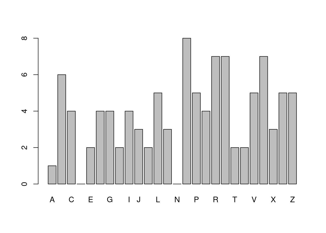
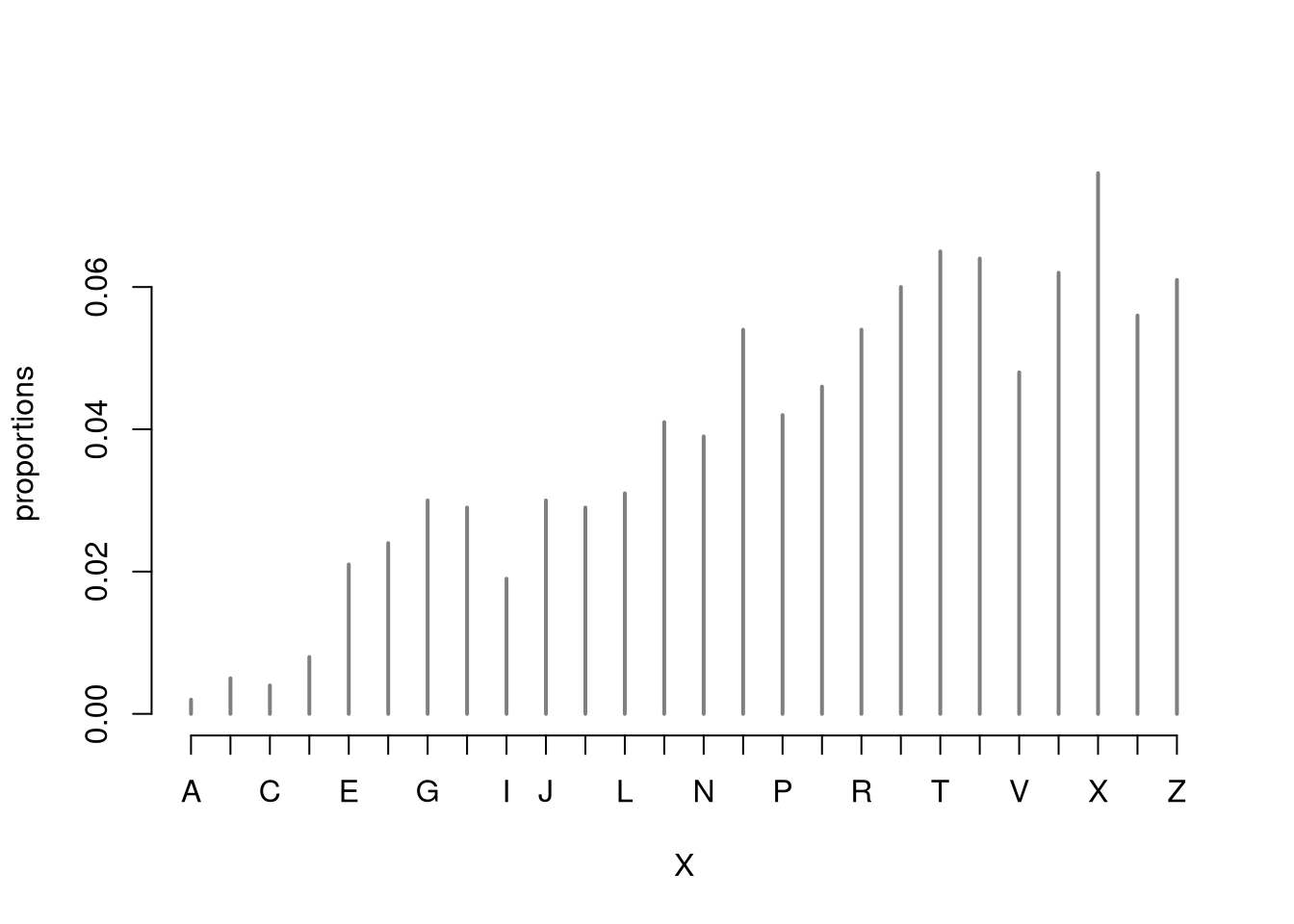
Mode and Share Concentration.

Sometimes, none of the above work well. With categorical data, for example, distributions are easier to describe with other statistics. The mode is the most common observation: the value with the highest observed frequency. We can also measure the spread of the frequencies or concentration at the mode vs elsewhere.

# Draw 3 Random Letters
x <- LETTERS
x_probs <- 1:length(x)
x_probs <- x_probs/sum(x_probs) # probs must sum to 1
X <- sample(x, 1, prob=x_probs, replace=T)
X
## [1] "V"

# Draw Random Letters 100 Times
X <- sample(x, 1000, prob=x_probs, replace=T)
X <- factor(unlist(X), levels=LETTERS, ordered=F)

proportions <- table(X)/length(X)
plot(proportions, col=grey(0,0.5))

# mode(s)
mode_id <- which(proportions==max(proportions))
names(proportions)[ mode_id ]
## [1] "X"

# freq. spreads
sd(proportions)
## [1] 0.02105655
sum(proportions^2)
## [1] 0.049546
# freq. concentration at mode
max(proportions)/mean(proportions)
## [1] 1.976

5.3 Shape Statistics

Central tendency and dispersion are often insufficient to describe a distribution. To further describe shape, we can compute skew and kurtosis to measure asymmetry and extreme values. There are many other statistics we could compute on an ad-hoc basis.

Skewness.

The skew statistic captures how asymmetric the distribution is by measuring the average cubed deviation from the mean, normalized the standard deviation cubed \[\begin{eqnarray} \frac{\sum_{i=1}^{n} [\hat{X}_{i} - \hat{M}]^3 / n}{ s^3 } \end{eqnarray}\]

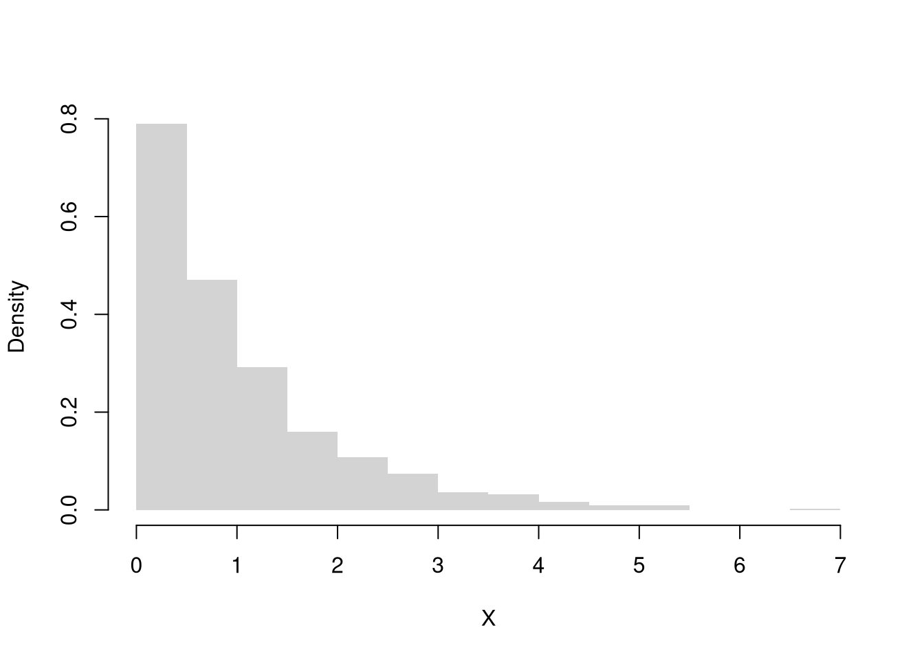
X <- rweibull(1000, shape=1)
hist(X, border=NA, main=NA, freq=F, breaks=20)

skewness <-  function(X){
 X_mean <- mean(X)
 m3 <- mean((X - X_mean)^3)
 s3 <- sd(X)^3
 skew <- m3/s3
 return(skew)
}

skewness( rweibull(1000, shape=1))
## [1] 2.052569
skewness( rweibull(1000, shape=10) )
## [1] -0.705397

We can automatically compare against the normal distribution, which has a skew of 0.

Kurtosis.

This statistic captures how many “outliers” there are like skew but looking at quartic deviations instead of cubed ones. \[\begin{eqnarray} \frac{\sum_{i=1}^{n} [\hat{X}_{i} - \hat{M}]^4 / n}{ s^4 }. \end{eqnarray}\] Some authors further subtract \(3\) to explicitly compare against the normal distribution (the normal distribution has a kurtosis of \(3\)).

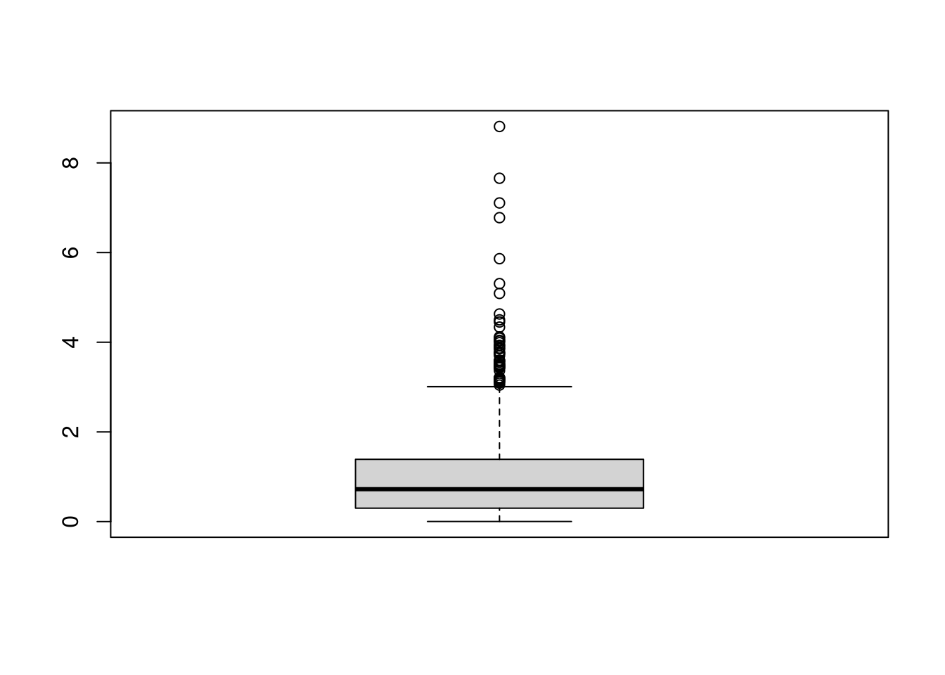
X <- rweibull(1000, shape=1)
boxplot(X, main=NA)

kurtosis <- function(X){  
 X_mean <- mean(X)
 m4 <- mean((X - X_mean)^4) 
 s4 <- sd(X)^4
 kurt <- m4/s4
 excess_kurt <- kurt - 3 # compare against normal
 return(kurt)
}

kurtosis( rweibull(1000, shape=1) )
## [1] 7.285463
kurtosis( rweibull(1000, shape=10) )
## [1] 3.348988

Clusters/Gaps.

You can also describe distributions in terms of how clustered the values are, including the number of modes, bunching, and many other statistics. But remember that “a picture is worth a thousand words”.

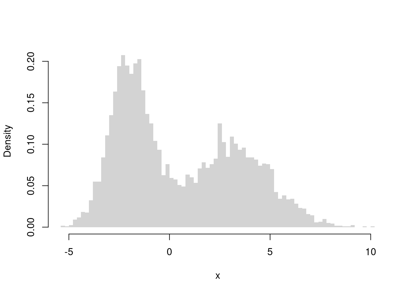
# Complicated Random Variable
r_ugly0 <- function(n, populationMean=c(-2, 3), populationVar=c(1, 4), prob=c(.5,.5)){
  # Which distribution is each observation coming from
  di <- sample(1:2, size=n, replace=TRUE, prob=prob)
  rnorm(n, mean=populationMean[di], sd=sqrt(populationVar)[di])
}

X <- r_ugly0(6000)
hist(X, breaks=60,
    freq=F, border=NA,
    xlab="x", main='')

#hist( rbeta(1000, .6, .6), border=NA, main=NA, freq=F, breaks=20)

# Another Complicated Random Variable
r_ugly1 <- function(n, theta1=c(-8,-1), theta2=c(-2,2), rho=.25){
    omega   <- rbinom(n, size=1, rho)
    epsilon <- omega * runif(n, theta1[1], theta2[1]) +
        (1-omega) * rnorm(n, theta1[2], theta2[2])
    return(epsilon)
}
# Very Large Sample
X <- r_ugly1(1000000)
hist(X, breaks=1000,  freq=F, border=NA,
    xlab="x", main='')

# Show True Density
d_ugly1 <- function(x, theta1=c(-8,-1), theta2=c(-2,2), rho=.25){
    rho     * dunif(x, theta1[1], theta2[1]) +
    (1-rho) * dnorm(x, theta1[2], theta2[2]) }
x <- seq(-12,6,by=.001)
dx <- d_ugly1(x)
lines(x, dx, col=1)

5.4 Probability Theory

You were already introduced to this with random variables. We will now dig a little deeper theoretically into the statistics we compute. When we know how the data are generated theoretically, we can often compute the theoretical value of the two most basic and often-used statistics: the mean and variance. To see this, we separately analyze how they are computed for discrete and continuous random variables.

Here, we denote \(X_{i}\) as a random variable that can take on specific values \(x\) from the sample space with known probabilities.

Discrete Random Variables.

If the sample space is discrete, we can compute the theoretical mean (or expected value) as \[\begin{eqnarray} \mathbb{E}[X_{i}] = \sum_{x} x Prob(X_{i}=x), \end{eqnarray}\] where \(Prob(X_{i}=x)\) is the probability the random variable \(X_{i}\) takes the particular value \(x\). Similarly, we can compute the theoretical variance as \[\begin{eqnarray} \mathbb{V}[X_{i}] = \sum_{x} \left(x - \mathbb{E}[X_{i}] \right)^2 Prob(X_{i}=x). \end{eqnarray}\] The theoretical standard deviation is \(\mathbb{s}[X_{i}] = \sqrt{\mathbb{V}[X_{i}]}\).

For example, consider a five-sided die with equal probability of landing on each side. I.e., \(X_{i}\) is a Discrete Uniform random variable with outcomes \(x \in \{1,2,3,4,5\}\). What is the theoretical mean? What is the variance and standard deviation? \[\begin{eqnarray} \mathbb{E}[X_{i}] &=& 1\frac{1}{5} + 2\frac{1}{5} + 3\frac{1}{5} + 4\frac{1}{5} + 5\frac{1}{5} = 15/5 = 3\\ \mathbb{V}[X_{i}] &=& (1-3)^2\frac{1}{5} + (2 - 3)^2\frac{1}{5} + (3 - 3)^2\frac{1}{5} + (4 - 3)^2\frac{1}{5} + (5 - 3)^2\frac{1}{5} \\ &=& 2^2 \frac{1}{5} + 1^2\frac{1}{5} + 0^2 \frac{1}{5} + + 1^2\frac{1}{5} + 2^2 \frac{1}{5} = (4 + 1 + 1 + 4)/5 = 10/5 = 2\\ \mathbb{s}[X_{i}] &=& \sqrt{2} \end{eqnarray}\]

# Computerized Way to Compute Mean
x <- c(1,2,3,4,5)
x_probs <- c(1/5, 1/5, 1/5, 1/5, 1/5)
X_mean <- sum(x*x_probs)
X_mean
## [1] 3

# Computerized Way to Compute SD
Xvar <- sum((x-X_mean)^2*x_probs)
Xvar
## [1] 2
Xsd <- sqrt(Xvar)
Xsd
## [1] 1.414214

# Verified by simulation
Xsim <- sample(x, prob=x_probs,
          size=10000, replace=T)
mean(Xsim)
## [1] 3.018
sd(Xsim)
## [1] 1.420168

Note

For example, consider an unfair coin with a \(3/4\) probability of heads (\(x=1\)) and a \(1/4\) probability of tails (\(x=0\)) has a theoretical mean of \[\begin{eqnarray} \mathbb{E}[X_{i}] = 0\frac{1}{4} + 1\frac{3}{4} = \frac{3}{4} \end{eqnarray}\] and a theoretical variance of \[\begin{eqnarray} \mathbb{V}[X_{i}] = [0 - \frac{3}{4}]^2 \frac{1}{4} + [1 - \frac{3}{4}]^2 \frac{3}{4} = \frac{9}{64} + \frac{3}{64} = \frac{12}{64} = \frac{3}{16}. \end{eqnarray}\] Verify both the mean and variance by simulation.

# A simulation of many coin flips
x <- c(0,1)
x_probs <- c(1/4, 3/4)
X <- sample(x, 1000, prob=x_probs, replace=T)

round( mean(X), 4)
## [1] 0.748

round( var(X), 4)
## [1] 0.1887

Note

Consider a four-sided die with outcomes \(\{1,2,3,4 \}\) and corresponding probabilities \(\{ 1/8, 2/8, 1/8, 4/8 \}\) . What is the mean? \[\begin{eqnarray} \mathbb{E}[X_{i}] = 1 \frac{1}{8} + 2 \frac{2}{8} + 3 \frac{1}{8} + 4 \frac{4}{8} = 3 \end{eqnarray}\] What is the variance? Verify both the mean and variance by simulation.

Tip

Consider an unfair coin with a \(p\) probability of heads (\(x=1\)) and a \(1-p\) probability of tails (\(x=0\)), where \(p\) is a parameter between \(0\) and \(1\). The theoretical mean is \[\begin{eqnarray} \mathbb{E}[X_{i}] = 1[p] + 0[1-p] = p \end{eqnarray}\] and the theoretical variance is \[\begin{eqnarray} \mathbb{V}[X_{i}] = [1 - p]^2 p + [0 - p]^2 [1-p] = [1 - p]^2 p + p^2 [1-p] = [1-p]p\left( [1-p] + p\right) = [1-p] p. \end{eqnarray}\] So the theoretical standard deviation is \(\mathbb{s}[X_{i}]=\sqrt{[1-p] p}\).

Tip

Suppose \(X_{i}\) is a discrete random variable with this probability mass function: \[\begin{eqnarray} X_{i} &=& \begin{cases} -1 & \text{ with probability } \frac{1}{2 \lambda^2} \\ 0 & \text{ with probability } 1-\frac{1}{\lambda^2} \\ +1 & \text{ with probability } \frac{1}{2\lambda^2} \end{cases}, \end{eqnarray}\] where \(\lambda>0\) is a parameter. What is the theoretical standard deviation?

Tip

For a discrete uniform random variable with th sample space \(\{1,2,3,4,5\}\), calculate the theoretical median and IQR.

Weighted Data.

Sometimes, you may have a dataset of values and probability weights. Othertimes, you can calculate them yourself. In either case, you can explicitly do the computations for discrete data. Given data on unique outcome \(x\) and their frequency \(\hat{p}_{x}=\sum_{i=1}^{n}\mathbf{1}\left(X_{i}=x\right)/n\), we compute \[\begin{eqnarray} \hat{M} &=& \sum_{x} x \hat{p}_{x}. \end{eqnarray}\]

Note

Suppose we flipped a coin \(100\) times and found that \(76\) were Heads and \(23\) were Tails. The estimated probabilities are \(76/100\) for the outcome \(X_{1}=1\) and \(24/100\) for the outcome \(X_{i}=0\). We compute the mean as \(\hat{M}=1\times 0.76 + 0 \times 0.24 = 0.76\).

# Compute a sample estimate using probability weights
P  <- table(X) #table of counts
p <- c(P)/length(X) #frequencies (must sum to 1)
x <- as.numeric(names(p)) #unique values
cbind(x,p)
##   x     p
## 0 0 0.252
## 1 1 0.748

# Sample Mean Estimate
X_mean <- sum(x*p)
X_mean
## [1] 0.748

Tip

Try estimating the sample mean the two different ways for another random sample

x <- c(0,1,2)
x_probs <- c(1/3,1/3,1/3)
X  <-  sample(x, prob=x_probs, 1000, replace=T)

# First Way (Computerized)
mean(X)
## [1] 0.932

# Second Way (Explicit Calculations)
# start with a table of counts like the previous example

This idea generalizes the mean to a weighted mean: an average where different values contribute to the final result with varying levels of importance. For each outcome \(x\) we have a weight \(W_{x}\) and compute \[\begin{eqnarray} \hat{M} &=& \frac{\sum_{x} x W_{x}}{\sum_{x} W_{x}} = \sum_{x} x w_{x}, \end{eqnarray}\] where \(w_{x}=\frac{W_{x}}{\sum_{x'} W_{x'}}\) is normalized version of \(W_{x}\) that implies \(\sum_{x}w_{x}=1\).¹

Note

For example, suppose a student has these scores

Homework1 <- c(score=88, weight=0.25)
Homework2 <- c(score=92, weight=0.25)
Exam1 <- c(score=67, weight=0.2)
Exam2 <- c(score=90, weight=0.3)

Grades <- rbind(Homework1, Homework2, Exam1, Exam2)
Grades
##           score weight
## Homework1    88   0.25
## Homework2    92   0.25
## Exam1        67   0.20
## Exam2        90   0.30

We can compute the final grade as a weighted mean

# Manual Way
88*0.25 + 92*0.25 + 67*0.2 + 90*0.3
## [1] 85.4

# Computerized Way
Values <- Grades[,'score'] * Grades[,'weight']
FinalGrade <- sum(Values)
FinalGrade
## [1] 85.4

The weighting idea generalizes to other statistics. E.g., we can also computed a weighted variance or weighted quantile.

Tip

Provide an example of computing a weighted variance building on this code below

x_diff <- (x - x_mean)^2
p <- P/sum(P)
x_var <- sum(p * x_diff)

See that we can also compute weighted quantiles

weighted.quantile <- function(x, w, probs){
    #See spatstat.univar::weighted.quantile
    oo <- order(x)
    x <- x[oo]
    w <- w[oo]
    Fx <- cumsum(w)/sum(w)
    quantile_id <- max(which(Fx <= probs))+1
    xq <- x[quantile_id] 
    return(xq)
}

## Unweighted
quantile(X, probs=.5)
## 50% 
##   1
weights <- rep(1, length(X))
weighted.quantile(x=X, w=weights, probs=.5)
## [1] 1

## Weighted
weights <- seq(X)
weights <- weights/sum(weights) # normalize
weighted.quantile(x=X, w=weights, probs=.5)
## [1] 1

Continuous Random Variables.

Many continuous random variables are parameterized by their means and variances. For example, the exponential distribution has parameter \(\lambda\), which corresponds to the theoretical mean \(1/\lambda\) and variance \(1/\lambda^2\). For another example, the two parameters of the normal distribution are \(\mu\) and \(\sigma\), which corresponds to the theoretical mean and variance.

# Exponential Random Variable
X <- rexp(5000, 2)
m <- mean(X)
round(m, 2)
## [1] 0.5

# Normal Random Variable
X <- rnorm(5000, 1, 2)
round(mean(X), 2)
## [1] 1.05
round(var(X), 2)
## [1] 4.11

Advanced and Optional

If the sample space is continuous, we can compute the theoretical mean (or expected value) as \[\begin{eqnarray} \mathbb{E}[X] = \int x f(x) d x, \end{eqnarray}\] where \(f(x)\) is the probability the random variable takes the particular value \(x\). Similarly, we can compute the theoretical variance as \[\begin{eqnarray} \mathbb{V}[X_{i}]= \int \left(x - \mathbb{E}[X_{i}] \right)^2 f(x) d x, \end{eqnarray}\]

For example, consider a random variable with a continuous uniform distribution over \([-1, 1]\). In this case, \(f(x)=1/[1 - (-1)]=1/2\) for each \(x \in [-1, 1]\) and \[\begin{eqnarray} \mathbb{E}[X_{i}] = \int_{-1}^{1} \frac{x}{2} d x = \int_{-1}^{0} \frac{x}{2} d x + \int_{0}^{1} \frac{x}{2} d x = 0 \end{eqnarray}\] and \[\begin{eqnarray} \mathbb{V}[X_{i}]= \int_{-1}^{1} x^2 \frac{1}{2} d x = \frac{1}{2} \frac{x^3}{3}|_{-1}^{1} = \frac{1}{6}[1 - (-1)] = 2/6 =1/3 \end{eqnarray}\]

X <- USArrests[,'Murder']
round( mean(X), 4)
## [1] 7.788
round( var(X), 4)
## [1] 18.9705

Tip

You can estimate means and variances for continuous random variables with weights, but here we have an additional approximation error

# values and probabilities
h  <- hist(X, plot=F)
wt <- h[['counts']]/length(X) 
xt <- h[['mids']]
# Weighted mean
X_mean <- sum(wt*xt)
X_mean
## [1] 7.8

# Compare to "mean(x)"

Try it yourself with

X <- runif(2000, -1, 1)

5.5 Further Reading

Probability Theory

• [Refresher] https://www.khanacademy.org/math/statistics-probability/probability-library/basic-theoretical-probability/a/probability-the-basics
• https://book.stat420.org/probability-and-statistics-in-r.html
• https://bookdown.org/speegled/foundations-of-statistics/
• https://math.dartmouth.edu/~prob/prob/prob.pdf
• https://bookdown.org/probability/beta/discrete-random-variables.html
• https://www.econometrics-with-r.org/2.1-random-variables-and-probability-distributions.html
• https://probability4datascience.com/ch02.html
• https://statsthinking21.github.io/statsthinking21-R-site/probability-in-r-with-lucy-king.html
• https://bookdown.org/probability/statistics/
• https://www.atmos.albany.edu/facstaff/timm/ATM315spring14/R/IPSUR.pdf
• https://rc2e.com/probability
• https://bookdown.org/probability/beta/
• https://bookdown.org/a_shaker/STM1001_Topic_3/
• https://bookdown.org/fsancier/bookdown-demo/
• https://bookdown.org/kevin_davisross/probsim-book/
• https://bookdown.org/machar1991/ITER/2-pt.html
• https://www.atmos.albany.edu/facstaff/timm/ATM315spring14/R/IPSUR.pdf
• https://math.dartmouth.edu/~prob/prob/prob.pdf

For weighted statistics, see

• https://seismo.berkeley.edu/~kirchner/Toolkits/Toolkit_12.pdf
• https://www.bookdown.org/rwnahhas/RMPH/survey-desc.html

---

1. Note that if there are \(K\) unique outcomes and \(W_{x}=1\) then \(\sum_{x}W_{x}=K\) and \(w_{x}=1/K\). This means \(\hat{M} = \sum_{x} x w_{x} = \sum_{x} x /K\), which is just a simple mean.