In this chapter, we test hypotheses using data-driven methods that assume much less about the data generating process. There are two main ways to conduct a hypothesis test: inverting a confidence interval and imposing the null. The first treats the distribution of estimates directly; the second explicitly enforces the null hypothesis to evaluate how unusual the observed statistic is. Both approaches rely on the bootstrap: resampling the data to approximate sampling variability. The most typical case is hypothesizing about the mean.
Invert a CI.
One main way to conduct hypothesis tests is to examine whether a confidence interval contains a hypothesized value. We then use this decision rule
reject the null if value falls outside of the interval
fail to reject the null if value falls inside of the interval
We typically use a \(95\%\) confidence interval to create a rejection region: the area that falls outside of the interval.
NoteMust Know
For example, suppose you hypothesize the mean is \(9\). You then construct a bootstrap distribution with \(95\%\) confidence interval, and find your hypothesized value falls outside of the confidence interval. Then, after accounting for sampling variability (which you estimate), it still seems extremely unlikely that the theoretical mean actually equals \(9\), so you reject that hypothesis. (If the theoretical value landed in the interval, you would “fail to reject” the theoretical mean equals \(9\).)
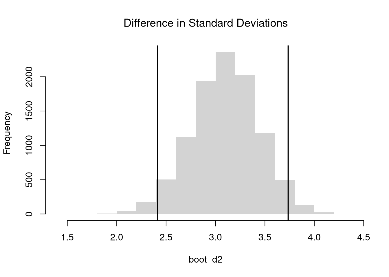
The above procedure also generalizes to many other statistics. Perhaps the most informative are those for spread or shape. E.g., you can conduct hypothesis tests for sd and IQR, or skew and kurtosis.
Code
# Bootstrap Distribution for SDsd_obs <-sd(sample_dat)bootstrap_sd <-rep(NA, 999)for(b inseq_along(bootstrap_sd)){ x_b <-sample(sample_dat, replace=T) sd_b <-sd(x_b) bootstrap_sd[b] <- sd_b}# Test for SD Differences (Invert CI)sd_null <-3.6hist(bootstrap_sd, freq=F,border=NA, xlab='Bootstrap',main=NA)title('Standard Deviations (Invert CI)', font.main=1)sd_ci <-quantile(bootstrap_sd, probs=c(0.025, .975) )abline(v=sd_ci, lwd=2)abline(v=sd_null, lwd=2, col=rgb(1, 0, 0, .8))
To better your understanding, try redoing the above for any function (such as IQR(x_b)/median(x_b))
TipTest Yourself
Suppose you scored \(83\%\) on your exam with \(50\) questions, but think you are really a \(90\%\) student. Explain how you might test your hypothesis to your professor who insists your claim be supported by evidence. What would be the issue if we could not reject your hypothesis? Provide a computer simulation illustrating the issue.
Impose the Null.
We can also compute a null distribution: the sampling distribution of the statistic under the null hypothesis (assuming your null hypothesis was true). We use the bootstrap to loop through a large number of “resamples”. In each iteration of the loop, we impose the null hypothesis and re-estimate the statistic of interest. We then calculate the range of the statistic across all resamples and compare how extreme the original value we observed is.
NoteMust Know
For example, suppose you hypothesize the mean is \(9\). You then construct a \(95\%\) confidence interval around the null bootstrap distribution (resamples centered around \(9\)). If your sample mean falls outside of that interval, then even after accounting for sampling variability (which you estimate), it seems extremely unlikely that the theoretical mean actually equals \(9\), so you reject that hypothesis. (If the sample mean landed in the interval, you would “fail to reject” the theoretical mean equals \(9\).)
Code
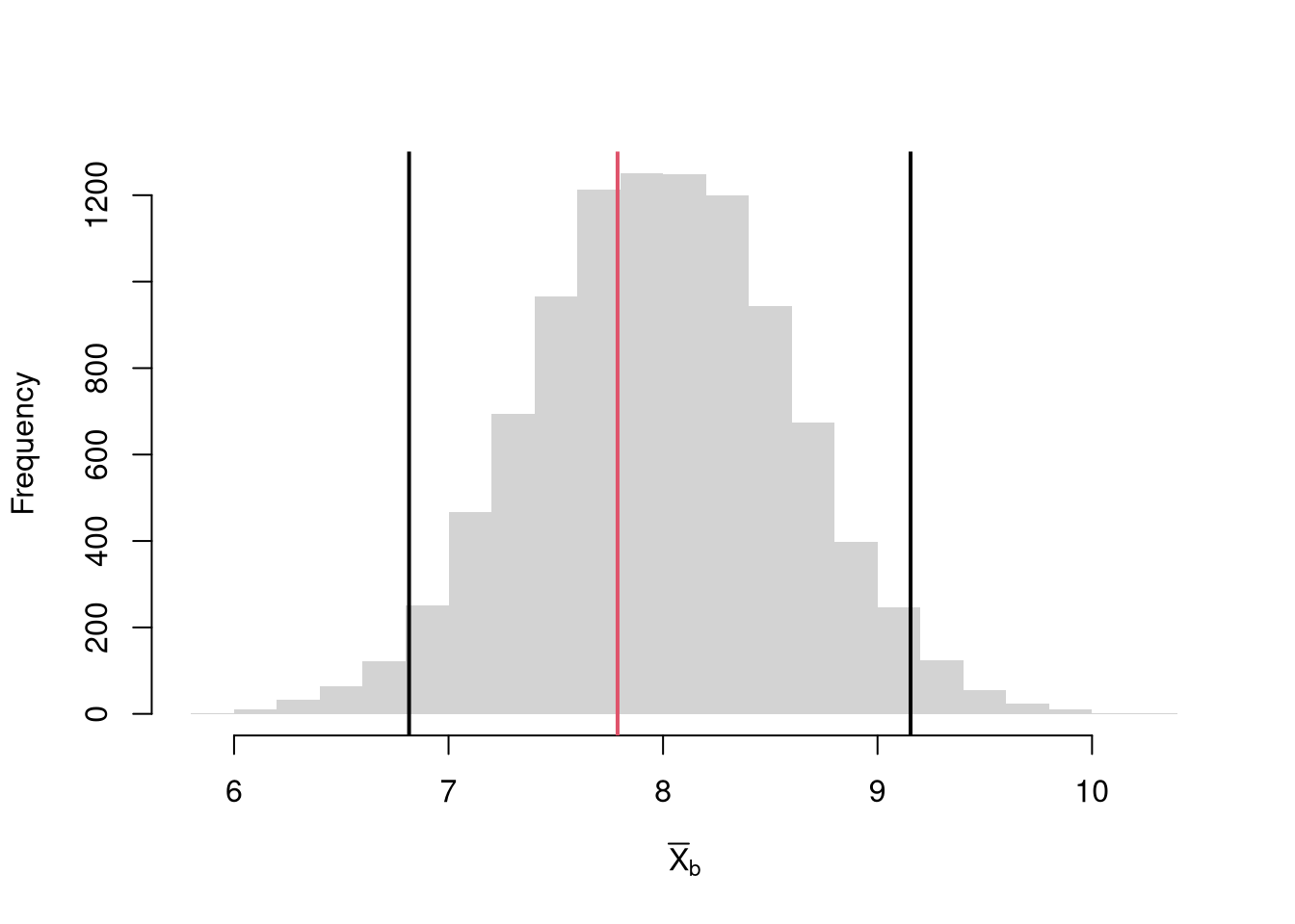
sample_dat <- USArrests[, 'Murder']sample_mean <-mean(sample_dat)# Bootstrap NULL: mean=9# Bootstrap shift: center each bootstrap resample so that the distribution satisfies the null hypothesis on average.set.seed(1)mu <-9bootstrap_means_null <-rep(NA, 999)for(b inseq_along(bootstrap_means_null)){ dat_b <-sample(sample_dat, replace=T) mean_b <-mean(dat_b) + (mu - sample_mean) # impose the null via Bootstrap shift bootstrap_means_null[b] <- mean_b}hist(bootstrap_means_null, breaks=25, border=NA, freq=F,main=NA,xlab='Null Bootstrap Samples')ci_95 <-quantile(bootstrap_means_null, probs=c(.025, .975)) # critical regionabline(v=ci_95, lwd=2)abline(v=sample_mean, lwd=2, col=rgb(0, 0, 1, .8))
The Normal approximation from the previous chapter can also impose the null: center the interval at the hypothesized value \(\mu\) and use \(\mu \pm q(\alpha/2) \cdot SE(M)\), where \(SE(M)\) is estimated via bootstrap or classical formulas. (While we could also use a Null Jackknife distribution, that is rarely done in practice.) Altogether, there are two different types of confidence intervals that “impose the null”. Until you know more, a conservative rule-of-thumb is to take the larger estimate.
Types of Confidence Interval Estimates that “impose the null”
Interval
Mechanism
Bootstrap (Percentile)
randomly resample \(n\) observations with replacement and shift
Normal
assume sampling distribution is Normal and use formula \(\pm q(\alpha/2) \cdot SE\)
8.2\(p\)-values
A \(p\)-value is the frequency you see something at least as extreme as your statistic under the null hypothesis (when sampling from the null distribution). We want the probability that the random variable \(M\) is at least as extreme (far from the null mean of \(9\)) as our observed sample mean \(\hat{M}\).
Recall that we used the bootstrap to estimate the distribution of the sample statistic like the mean, and the null-bootstrap shifted the bootstrap to be centered at a hypothesized value. The bootstrap idea here is to approximate \(M-\mu\), the difference between the sample mean \(M\) and the unknown theoretical mean \(\mu\), with the null-bootstrap analogue \(M^{\text{boot}}_{0}-\mu\), where \(M^{\text{boot}}_{0}=M^{\text{boot}}+(\mu-\hat{M})\) is the recentered bootstrap mean. \[\begin{eqnarray}
& & Prob( |M - \mu| \geq |\hat{M} - \mu| \mid \mu = 9 ) \\
& & \approx Prob( |M^{\text{boot}}_{0}- \mu| \geq |\hat{M}- \mu| \mid \mu = 9) \\
& & = 1-\hat{F}^{|\text{boot}|}_{0}(|\hat{M}-9|),
\end{eqnarray}\] where \(\hat{F}^{|\text{boot}|}_{0}\) is the ECDF of \(|M^{\text{boot}}_{0}- \mu|\).
NoteMust Know
(Repeating the null bootstrap from above for reference.)
Code
sample_dat <- USArrests[, 'Murder']sample_mean <-mean(sample_dat)set.seed(1)# Bootstrap NULL: mean=9# Bootstrap shift: center each bootstrap resample so that the distribution satisfies the null hypothesis on average.mu <-9bootstrap_means_null <-rep(NA, 999)for(b inseq_along(bootstrap_means_null)){ dat_b <-sample(sample_dat, replace=T) mean_b <-mean(dat_b) + (mu - sample_mean) # impose the null via Bootstrap shift bootstrap_means_null[b] <- mean_b}hist(bootstrap_means_null, breaks=25, border=NA, freq=F,main=NA,xlab='Null Bootstrap Samples')ci_95 <-quantile(bootstrap_means_null, probs=c(.025, .975)) # critical regionabline(v=ci_95, lwd=2)abline(v=sample_mean, lwd=2, col=rgb(0, 0, 1, .8))
Code
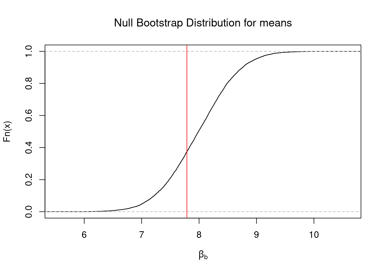
# Two-Sided Test, ALTERNATIVE: mean < 9 or mean >9# Visualize Two Sided Prob. & reject region boundarypar(mfrow=c(1, 2))hist(bootstrap_means_null-mu,freq=F, breaks=20,border=NA,main=NA,xlab=expression('Null Bootstrap for M - '~mu))abline(v=sample_mean-mu, col=rgb(0, 0, 1, .8))ci_95 <-quantile(bootstrap_means_null-mu, probs=c(0.025, .975))abline(v=ci_95, lwd=2)# Equivalent Visualizationboot_absval <-abs(bootstrap_means_null-mu)Fhat_abs0 <-ecdf(boot_absval)plot(Fhat_abs0,main=NA,xlab=expression('Null Bootstrap for |M - '~mu~'|'))abline(v=abs(sample_mean-mu), col=rgb(0, 0, 1, .8))# with Two Sided Probabilityp2 <-1-Fhat_abs0( abs(sample_mean-mu) )title( paste0('p=', round(p2, 3)), font.main=1)
You can conduct hypothesis test using \(p\)-values instead of confidence intervals. It is common to use this decision rule:
reject the null at the \(5\%\) level if \(p \leq 0.05\)
fail to reject the null at the \(5\%\) level if \(p > 0.05\)
Caveats.
Beware that a common misreading of the \(p\)-value as “the probability the null is true”. That is false. A \(p\)-value is the frequency you see something at least as extreme as your statistic under the null hypothesis.
Often, one may also see or hear “\(p<.05\): statistically significant” and “\(p>.05\): not statistically significant”. That is decision making on purely statistical grounds, and it may or may not be suitable for your context. You simply need to know that whoever says those things is using \(5\%\) as a critical value to reject a null hypothesis.
Code
# Purely-Statistical Decision Making# via Two Sided Testif(p2 >.05){print('fail to reject the null that mean=9, at the 5% level')} else {print('reject the null that mean=9 in favor of either <9 or >9, at the 5% level')}## [1] "reject the null that mean=9 in favor of either <9 or >9, at the 5% level"
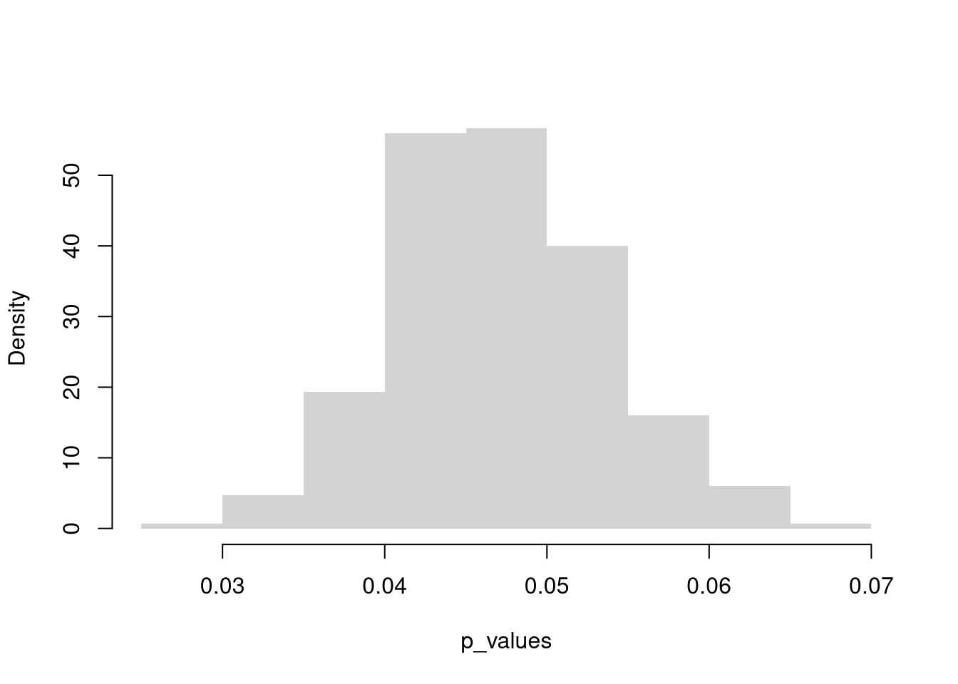
Also note that the \(p\)-value is itself a function of data, and hence a random variable that changes from sample to sample. Given that the \(5\%\) level is somewhat arbitrary, and that the \(p\)-value both varies from sample to sample and is often misunderstood, it makes sense to give specific \(p\)-values a limited role in decision making.
A \(t\)-value standardizes the approach for hypothesis tests of the mean. \[\begin{eqnarray}
t = (M - \mu) / SE(M),
\end{eqnarray}\]
For any specific sample, we must approximate the standard error. Using the theory-driven approach, we compute \(\hat{t}=(\hat{M}-\mu)/(\hat{S}/\sqrt{n})\). Using the data-driven approach, we compute \(\hat{t}=(\hat{M}-\mu)/(\hat{SE}^{\text{jack}})\) or \(\hat{t}=(\hat{M}-\mu)/(\hat{SE}^{\text{boot}})\). In any case, we can use bootstrapping to estimate the variability of the \(t\) statistic, just like we did with the mean.
NoteMust Know
Code
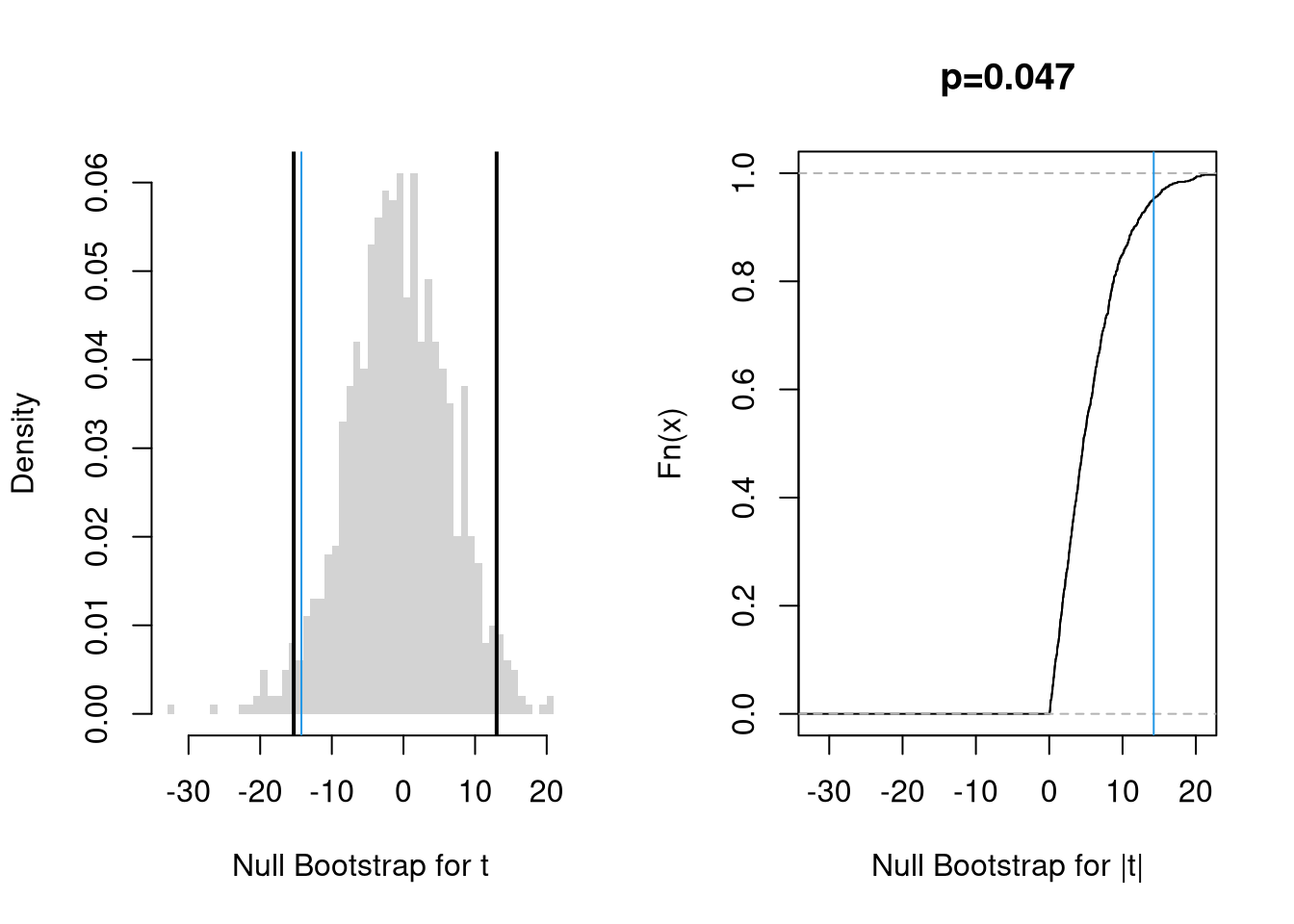
#null hypothesismu <-9# t statisticjackknife_means <-rep(NA, length(sample_dat))for(i inseq_along(jackknife_means)){ dat_i <- sample_dat[-i] jackknife_means[i] <-mean(dat_i)}jackknife_se <-sd(jackknife_means)*sqrt(length(sample_dat))sample_t <- (sample_mean - mu)/jackknife_se# Boostrap Null Distributionbootstrap_t_null <-rep(NA, 999)for(b inseq_along(bootstrap_t_null)){ dat_b <-sample(sample_dat, replace=T) mean_b <-mean(dat_b) + (mu - sample_mean) # impose the null by recentering# Compute t stat using jackknife ses (same as above) jackknife_means_b <-rep(NA, length(dat_b))for(i inseq_along(jackknife_means_b)){ jackknife_means_b[i] <-mean(dat_b[-i]) } jackknife_se_b <-sd(jackknife_means_b)*sqrt(length(dat_b)) jackknife_t_b <- (mean_b - mu)/jackknife_se_b bootstrap_t_null[b] <- jackknife_t_b}# Plot the null distribution and CIpar(mfrow=c(1, 2))hist(bootstrap_t_null, border=NA, breaks=50,freq=F, main=NA, xlab='Null Bootstrap for t')abline(v=sample_t, col=rgb(0, 0, 1, .8))ci_95 <-quantile(bootstrap_t_null, probs=c(0.025, 0.975) )abline(v=ci_95, lwd=2)# Compute the p-value for two-sided testFhat0 <-ecdf(abs(bootstrap_t_null))plot(Fhat0,xlim=range(bootstrap_t_null, sample_t),xlab='Null Bootstrap for |t|',main=NA)abline(v=abs(sample_t), col=rgb(0, 0, 1, .8))p <-1-Fhat0( abs(sample_t) )title( paste0('p=', round(p, 3)), font.main=1)
Code
if(p >.05){print('fail to reject the null that mean=9, at the 5% level')} else {print('reject the null that mean=9 in favor of either <9 or >9, at the 5% level')}## [1] "fail to reject the null that mean=9, at the 5% level"
There are several benefits to this statistic:
uses the same statistic for different hypothesis tests
makes the statistic comparable across different studies
removes dependence on unknown parameters by normalizing with a standard error
makes the null distribution theoretically known asymptotically (approximately)
The last point implies we are typically dealing with a normal distribution that is well-studied, or another well-studied distribution derived from it. We will discuss this more when comparing means.
Quantiles and Shape Statistics.
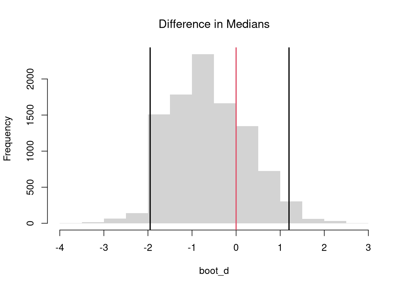
Bootstrap allows hypothesis tests for any statistic, not just the mean, without relying on parametric theory. For example, the above procedures generalize from means to quantile statistics like medians.
Code
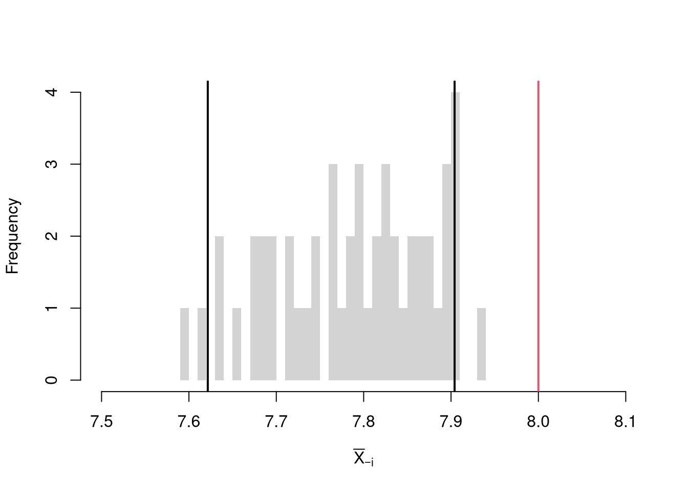
# Test for Median Differences (Impose the Null)# Bootstrap Null Distribution for the median# Each Bootstrap shifts medians so that median = q_nullq_obs <-quantile(sample_dat, probs=.5)q_null <-7.8bootstrap_quantile_null <-rep(NA, 999)for(b inseq_along(bootstrap_quantile_null)){ x_b <-sample(sample_dat, replace=T) #bootstrap sample q_b <-quantile(x_b, probs=.5) # median q_b_null <- q_b + (q_null - q_obs) # impose the null bootstrap_quantile_null[b] <- q_b_null}# 2-Sided Test for Medianshist(bootstrap_quantile_null-q_null,border=NA, freq=F, xlab='Null Bootstrap',main=NA)title('Medians (Impose Null)', font.main=1)median_ci <-quantile(bootstrap_quantile_null-q_null, probs=c(.025, .975))abline(v=median_ci, lwd=2)abline(v=q_obs-q_null, lwd=2, col=rgb(0, 0, 1, .8))
Code
# 2-Sided Test for Median Difference## Null: No Median Difference1-ecdf( abs(bootstrap_quantile_null-q_null))( abs(q_obs-q_null) )## [1] 0.5695696
TipTest Yourself
Conduct a hypothesis test for whether the upper quartile is statistically different from \(12\).
Code
q_obs <-quantile(sample_dat, probs=.75)
8.4 One-Sided Tests
Above, we tested whether the observed statistic is either extremely high or low. This is known as a two-sided test. There are also two one-sided tests (left tail: observed statistic is extremely low, right tail: observed statistic is extremely high). For a concrete example, consider whether the mean statistic, \(M\), is centered on a theoretical value of \(\mu=9\) for the population. If your null hypothesis is that the theoretical mean is nine, \(H_{0}: \mu =9\), and you calculated the mean for your sample as \(\hat{M}\), then you can consider any one of these three alternative hypotheses:
\(H_{A}: \mu \neq 9\), a two-tail test
\(H_{A}: \mu < 9\), a left-tail test
\(H_{A}: \mu > 9\), a right-tail test
One-sided hypothesis tests can be conducted by inverting a one-sided confidence interval (covered in the previous chapter) or by computing a one-sided \(p\)-value.
One-Sided \(p\)-values.
The \(p\)-value for a one-sided test is more straightforward to implement via a bootstrap null distribution.
For a left-tail test, we examine \[\begin{eqnarray}
p = Prob( M < \hat{M} \mid \mu = 9 )
&\approx& Prob( M^{\text{boot}} < \hat{M} \mid \mu = 9 ) = \hat{F}^{\text{boot}}_{0}(\hat{M}),
\end{eqnarray}\] where \(\hat{F}^{\text{boot}}_{0}\) is the ECDF of the bootstrap null distribution. We reject the null if \(p < 0.05\) at the \(5\%\) level, and otherwise fail to reject.
For a right-tail test, we examine \(p=Prob( M > \hat{M} \mid \mu = 9 ) \approx 1-\hat{F}^{\text{boot}}_{0}(\hat{M})\).
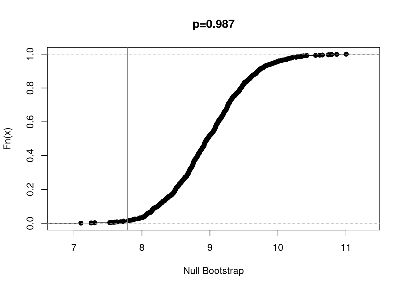
Code
# Right-tail Test, ALTERNATIVE: mean > 9# Equivalent Visualization with p-valueFhat0 <-ecdf(bootstrap_means_null) # Look at right tailplot(Fhat0,main=NA,xlab='Null Bootstrap')abline(v=sample_mean, col=rgb(0, 0, 1, .8))p1 <-1-Fhat0(sample_mean) #Compute right tail prob: 0.987title( paste0('p=', round(p1, 3)), font.main=1)
Code
if(p1 >.05){print('fail to reject the null that mean=9, at the 5% level')} else {print('reject the null that mean=9 in favor of >9, at the 5% level')}## [1] "fail to reject the null that mean=9, at the 5% level"
TipTest Yourself
Notice that the recentering adjustment affects two-sided tests (because they depend on distance from the null mean) but not one-sided tests (because adding a constant does not change rank order). Specifically, \(p = Prob( M < \hat{M} \mid \mu = 9 ) = Prob( M - \mu < \hat{M} - \mu \mid \mu = 9 )\). That is intuitively also why the \(t\)-value can be used for both one and two-sided hypothesis tests.
Code
# See that the 'recentering' matters for two-sided testsecdf( abs(bootstrap_means_null-mu) )( abs(sample_mean-mu) )## [1] 0.966967ecdf( abs(bootstrap_means_null) )( abs(sample_mean) )## [1] 0.01301301# See that the 'recentering' doesn't matter for one-sided onesecdf( bootstrap_means_null-mu)( sample_mean-mu)## [1] 0.01301301ecdf( bootstrap_means_null )( sample_mean)## [1] 0.01301301
8.5 Exercises
Explain the difference between “rejecting the null hypothesis” and “proving the alternative hypothesis is true.” Why is the phrase “fail to reject” used instead of “accept the null”?
Suppose you collect a sample of \(n = 50\) observations with \(\hat{M} = 22.4\) and \(\hat{S} = 6.0\). You want to test \(H_{0}: \mu = 20\) against \(H_{A}: \mu \neq 20\) at the \(5\%\) level. Compute the \(t\)-value using theory-driven standard errors and determine whether you reject or fail to reject.
Using the USArrests dataset in R, test the hypothesis that the population mean of Assault equals \(150\) by constructing a bootstrap null distribution. Compute the two-sided \(p\)-value and state whether you reject or fail to reject at the \(5\%\) level.