The two basic types of data are cardinal (aka numeric) data and factor data. We can further distinguish between whether cardinal data are discrete or continuous. We can also further distinguish between whether factor data are ordered or not
Cardinal (Numeric): the difference between elements always means the same thing.
Discrete: E.g. \(\{ 1,2,3\}\) and notice that \(2-1=3-2\).
Continuous: E.g., \(\{1.4348, 2.4348, 2.9, 3.9 \}\) and notice that \(2.9-1.4348=3.9-2.4348\)
Factor: the difference between elements does not always mean the same thing.
Ordered: E.g., \(\{1^{st}, 2^{nd}, 3^{rd}\}\) place in a race and notice that \(1^{st}\) - \(2^{nd}\) place does not equal \(2^{nd}\) - \(3^{rd}\) place for a very competitive person who cares only about winning.
Unordered (categorical): E.g., \(\{Amanda, Bert, Charlie\}\) and notice that \(Amanda - Bert\) never makes sense.
Here are some examples
Code
dat_card1 <-c(1,2,3) # Cardinal data (Discrete)dat_card1## [1] 1 2 3dat_card2 <-c(1.1, 2/3, 3) # Cardinal data (Continuous)dat_card2## [1] 1.1000000 0.6666667 3.0000000dat_fact1 <-factor( c('A','B','C'), ordered=T) # Factor data (Ordinal)dat_fact1## [1] A B C## Levels: A < B < Cdat_fact2 <-factor( c('Leipzig','Los Angeles','Logan'), ordered=F) # Factor data (Categorical)dat_fact2## [1] Leipzig Los Angeles Logan ## Levels: Leipzig Logan Los Angelesdat_fact3 <-factor( c(T,F), ordered=F) # Factor data (Categorical)dat_fact3## [1] TRUE FALSE## Levels: FALSE TRUE# Explicitly check the data types:#class(dat_card1)#class(dat_card2)
Note that for theoretical analysis, the types are sometimes grouped differently as
Discrete (discrete cardinal, ordered factor, and unordered factor data). You can count the potential values. E.g., the set \(\{A,B,C\}\) has three potential values.
Continuous (continuous cardinal data). There are uncountably infinite potential values. E.g., Try counting the numbers between \(0\) and \(1\) including decimal points, and notice that any two numbers have another potential number between them.
In any case, data are often computationally analyzed as data.frame objects, discussed below.
Strings.
Note that R allows for unstructured plain text, called character strings, which we can then format as factors
Code
c('A','B','C') # character strings## [1] "A" "B" "C"c('Leipzig','Los Angeles','Logan') # character strings## [1] "Leipzig" "Los Angeles" "Logan"
Also note that strings are encounter in a variety of settings, and you often have to format them after reading them into R.1
Code
# Stringspaste( 'hi', 'mom')## [1] "hi mom"paste( c('hi', 'mom'), collapse='--')## [1] "hi--mom"kingText <-"The king infringes the law on playing curling."gsub(pattern="ing", replacement="", kingText)## [1] "The k infres the law on play curl."# advanced usage#gsub("[aeiouy]", "_", kingText)#gsub("([[:alpha:]]{3})ing\\b", "\\1", kingText)
3.2 Datasets
Datasets can be stored in a variety of formats on your computer. But they can be analyzed in R in three basic ways.
A data.frame looks like a matrix but each column is actually a list rather than a vector. This allows you to combine different data types into a single object for analysis, which is why it might be your most common object.
Code
# data.frames: your most common data type# matrix of different data-types# well-ordered listsdata.frame(x, y) # list of vectors## x y## 1 1 2## 2 2 4## 3 3 6## 4 4 8## 5 5 10## 6 6 12## 7 7 14## 8 8 16## 9 9 18## 10 10 20
Note
Create a data.frame storing two different types of data. Then show print only the second column
Code
d0 <-data.frame(x=dat_fact2, y=dat_card2)d0## x y## 1 Leipzig 1.1000000## 2 Los Angeles 0.6666667## 3 Logan 3.0000000d0[,'y']## [1] 1.1000000 0.6666667 3.0000000
Arrays.
Arrays are generalization of matrices to multiple dimensions. They are a very efficient way to store well-formatted numeric data, and are often used in spatial econometrics and time series (often in the form of “data cubes”).
Regardless of the data types you have, you typically begin by inspecting your data by examining the first few observations.
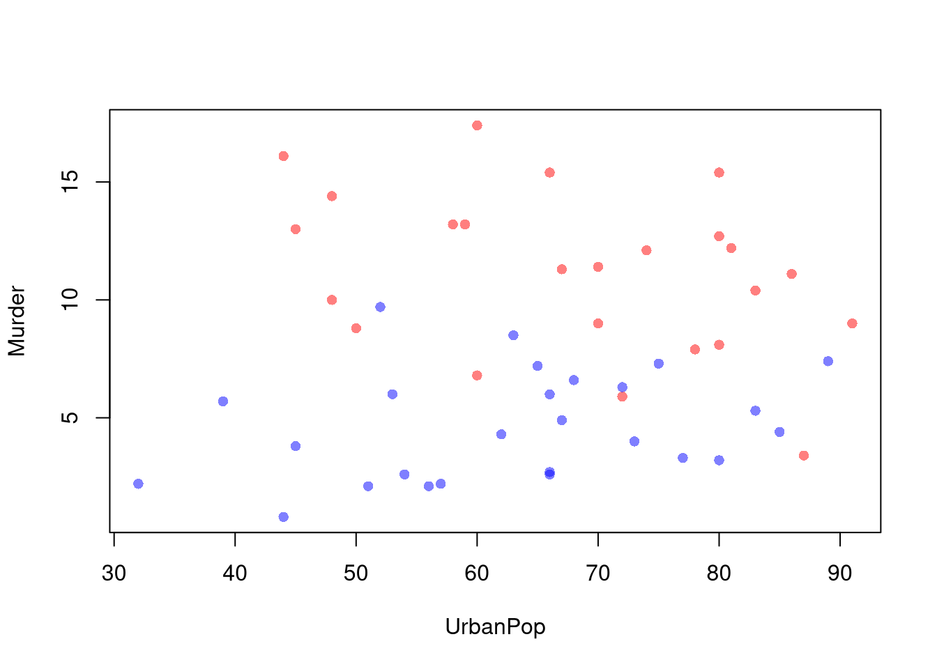
Consider, for example, historical data on crime in the US.
Code
head(USArrests) # Actual Data## Murder Assault UrbanPop Rape## Alabama 13.2 236 58 21.2## Alaska 10.0 263 48 44.5## Arizona 8.1 294 80 31.0## Arkansas 8.8 190 50 19.5## California 9.0 276 91 40.6## Colorado 7.9 204 78 38.7# Check NA valuesX <-c(3,3.1,NA,0.02) #Small dataset we will use in numerical examplessum(is.na(X))## [1] 1
To further examine a particular variable, we look at its distribution. In what follows, we will often work with data as vector \(\hat{X}=(\hat{X}_{1}, \hat{X}_{2}, ....\hat{X}_{n})\), where there are \(n\) observations and \(\hat{X}_{i}\) is the value of the \(i\)th one. We often analyze observations in comparison to some value \(x\).
The histogram measures the proportion of the data in different bins. It does so by dividing the range of the data into exclusive bins of equal-width \(h\), and count the number of observations within each bin. We often rescale the counts, dividing by the number of observations \(n\) multiplied by bin-width \(h\), so that the total area of the histogram sums to one, which allows us to interpret the numbers as a density.
Mathematically, for an exclusive bin \(\left(x-\frac{h}{2}, x+\frac{h}{2} \right]\) defined by their midpoint \(x\) and width \(h\), we compute \[\begin{eqnarray}
\hat{f}(x) &=& \frac{ \sum_{i=1}^{n} \mathbf{1}\left( \hat{X}_{i} \in \left(x-\frac{h}{2}, x+\frac{h}{2} \right] \right) }{n h},
\end{eqnarray}\] where \(\mathbf{1}()\) is an indicator function that equals \(1\) if the expression inside is TRUE and \(0\) otherwise. E.g., if \(\hat{X}_{i}=3.8\) and \(h=1\), then for \(x=1\) we have \(\mathbf{1}\left( \hat{X}_{i} \in \left(1-\frac{h}{2}, 1+\frac{h}{2} \right] \right)=\mathbf{1}\left( 3.8 \in \left(0.5, 1.5\right] \right)=0\) and for \(x=4\)\(\mathbf{1}\left( \hat{X}_{i} \in \left(4-\frac{h}{2}, 4+\frac{h}{2} \right] \right)=\mathbf{1}\left( 3.8 \in \left(3.5, 4.5\right] \right)=1\).
Note that the area of the rectangle is “base x height”, which is \(h \times \hat{f}(x)= \sum_{i=1}^{n} \mathbf{1}\left( \hat{X}_{i} \in \left(x-\frac{h}{2}, x+\frac{h}{2} \right] \right) /n\). This means the rectangle area equals the proportion of data in the bin. We compute \(\hat{f}(x)\) for each bin midpoint \(x\), and the area of all rectangles sums to one. 2
Note
For example, consider the dataset \(\{3,3.1,0.02\}\) and use bins \((0,1], (1,2], (2,3], (3,4]\). In this case, the midpoints are \(x=(0.5,1.5,2.5,3.5)\) and \(h=1\). Then the counts at each midpoints are \((1,0,1,1)\). Since \(\frac{1}{nh}=\frac{1}{3\times1}=\frac{1}{3}\), we can rescale the counts to compute the density as \(\hat{f}(x)=(1,0,1,1) \frac{1}{3}=(1/3,0,1/3,1/3)\).
For another example, use the bins \((0,2]\) and \((2,4]\). So the midpoints are \(1\) and \(3\), and the bin width is \(2\). Only one observation, \(0.02\), falls in the bin \((0,2]\). The other two observations, \(3\) and \(3.1\), fall into the bin \((2,4]\). The scaling factor is \(\frac{1}{nh}=\frac{1}{3\times 2}=\frac{1}{6}\). So the first bin has density \(f(1)=1\frac{1}{6}=1/6\) and the second bin has density \(f(3)=2\frac{1}{6}=2/6\). The area of the first bin’s rectangle is \(2 \times f(1)=2/6=1/3\) and the area of the second rectangle is \(2 \times f(3)=4/6=2/3\).
Now intuitively work through an example with three bins instead of four. Compute the areas
Code
Xhist <-hist(X, breaks=c(0,4/3,8/3,4), plot=F)base <-4/3height <- Xhist$densitysum(base*height)## [1] 1# as a default, R uses bins (,] instead of [,)# but you can change that with "right=F"# hist(X, breaks=c(0,4/3,8/3,4), plot=F, right=F)
# Since h=1, the density equals the proportion of states in each bin# Redo this example with h=2
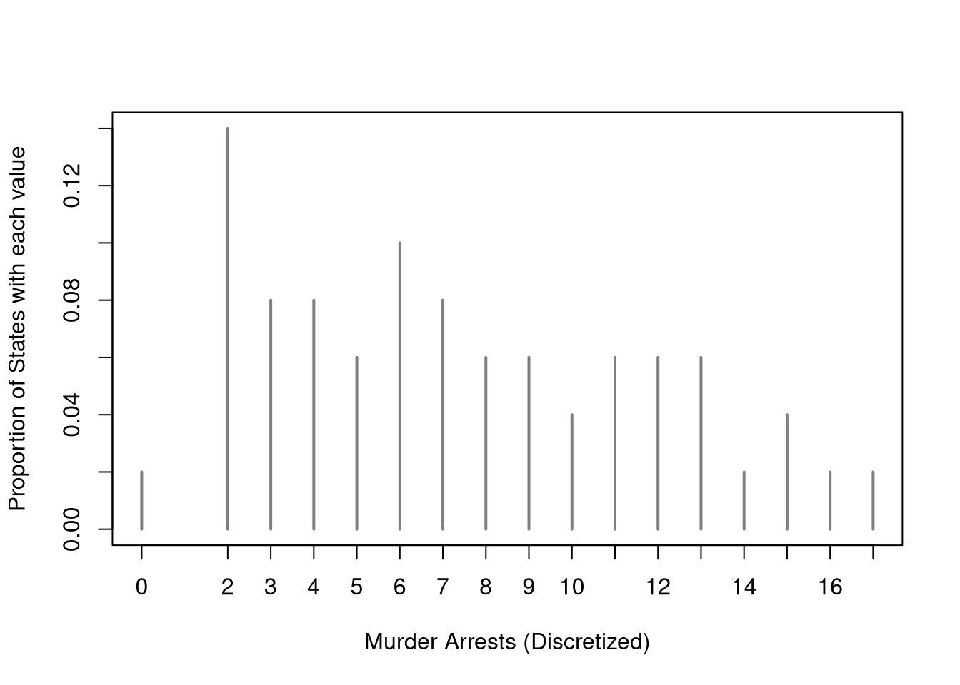
Note that if you your data are factor data, or discrete cardinal data, you can directly plot the proportions in a bar plot. For each unique outcome \(x\) we compute \[\begin{eqnarray}
\hat{p}_{x}=\sum_{i=1}^{n}\mathbf{1}\left(\hat{X}_{i}=x\right)/n.
\end{eqnarray}\] where \(n\) is the number of observations and \(\sum_{i=1}^{n}\mathbf{1}\left(\hat{X}_{i}=x\right)\) counts the number of observations equal to \(x\). The height of each line equals the proportion of data with a specific value.
Code
# Discretized dataX <- USArrests[,'Murder']Xr <-floor(X) #rounded down#table(Xr)proportions <-table(Xr)/length(Xr)plot(proportions, col=grey(0,.5),xlab='Murder Arrests (Discretized)',ylab='Proportion of States with each value')
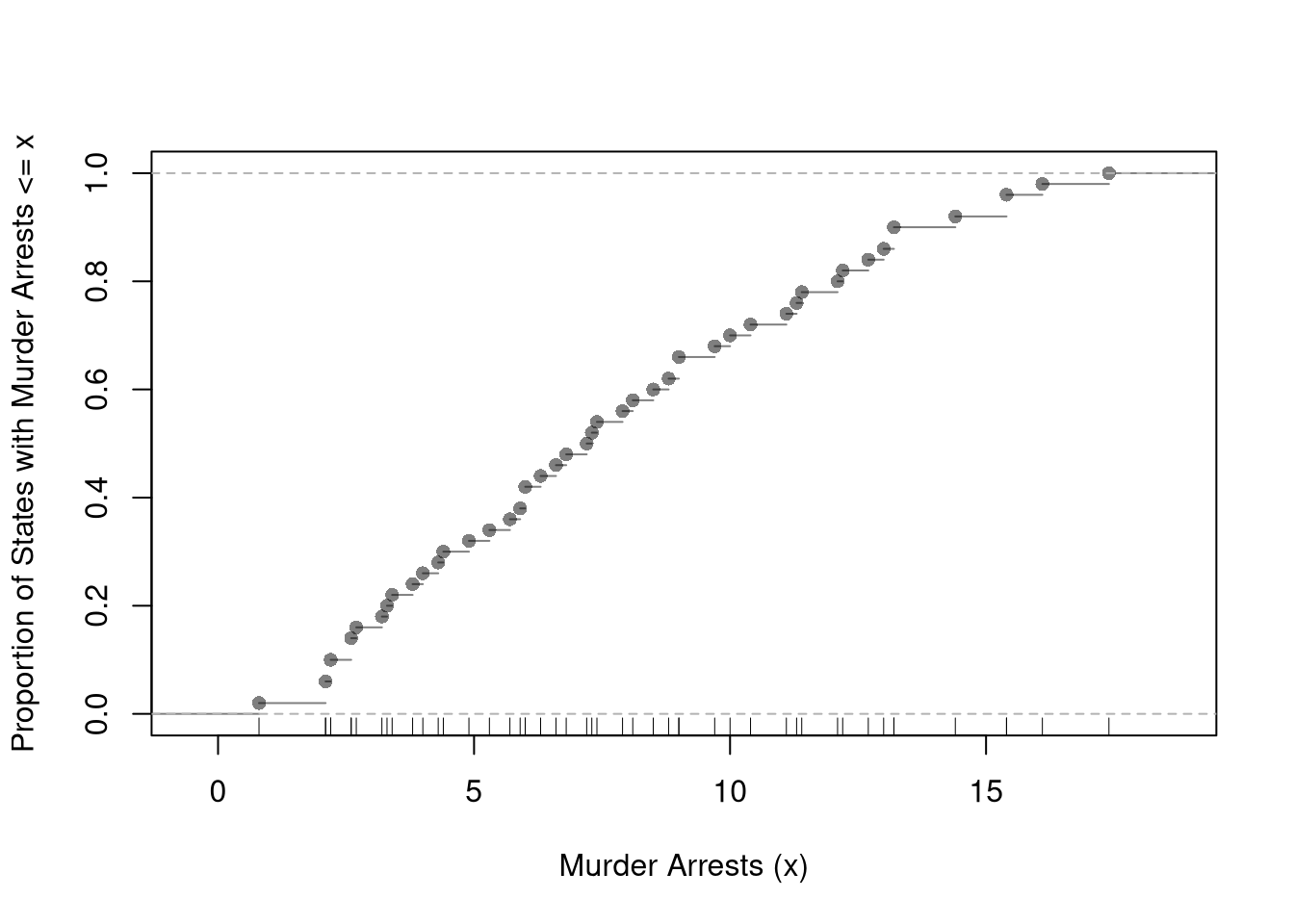
Empirical Cumulative Distribution Function.
The ECDF counts the proportion of observations whose values are less than or equal to \(x\); \[\begin{eqnarray}
\hat{F}(x) = \frac{1}{n} \sum_{i}^{n} \mathbf{1}( \hat{X}_{i} \leq x).
\end{eqnarray}\] Typically, we compute this for each unique value of \(x\) in the dataset. The ECDF jumps up by \(1/n\) at each of the \(n\) data points.
Note
For example, let \(X=(3,3.1,0.02)\). We reorder the observations as \((0.02, 3, 3.1)\), so that there are discrete jumps of \(1/n=1/3\) at each value. Consider the points \(x \in \{0.5,2.5,3.5\}\). At \(x=0.5\), \(F(0.5)\) measures the proportion of the data \(\leq 0.5\). Since only one observations, \(0.02\), of three is \(\leq 0.5\), we can compute \(F(0.5)=1/3\). Similarly, since only one observations, \(0.02\), of three is \(\leq 2.5\), we can compute \(F(2.5)=1/3\). Since all observations are \(\leq 3.5\), we can compute \(F(3.5)=1\).
Code
X <-c(3,3.1,0.02)Fhat <-ecdf(X)# Visualizedplot(Fhat)
Code
# Evaluated at the datax <- XFhat(X)## [1] 0.6666667 1.0000000 0.3333333#sum(X<=3)/length(X)#sum(X<=3.1)/length(X)#sum(X<=0.02)/length(X)# Evaluated at other pointsx <-c(0.5, 2.5, 3.5)Fhat(x)## [1] 0.3333333 0.3333333 1.0000000#sum(X<=0.5)/length(X)#sum(X<=2.5)/length(X)#sum(X<=3.5)/length(X)
Code
F_murder <-ecdf(USArrests[,'Murder'])# proportion of murders <= 10F_murder(10)## [1] 0.7# proportion of murders <= x, for all xplot(F_murder, main='', xlab='Murder Arrests (x)',ylab='Proportion of States with Murder Arrests <= x',pch=16, col=grey(0,.5))rug(USArrests[,'Murder'])
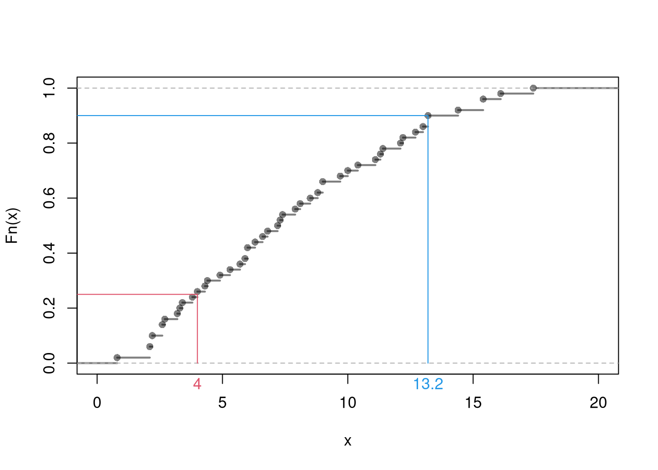
Quantiles.
You can summarize the distribution of data using quantiles: the \(p\)th quantile is a value of \(x\) where \(p\) percent of the data are below \(x\) and (\(1-p\)) percent are above \(x\).
The min is the smallest value (or the most negative value if there are any), where \(0%\) of the data has lower values.
The median is the middle value, where one half of the data has lower values and the other half has higher values.
The max is the smallest value (or the most negative value if there are any), where \(100%\) of the data has lower values.
Note
For example, if \(X=(0,0,0.02,3,5)\) then the median is \(0.02\), the lower quartile is \(0\), and the upper quartile is \(3\). (The number \(0\) is also special: the most frequent observation is called the mode.)
Now work through an intuitive example with observations \(\{1,2,...,13\}\). Hint: split the ordered observations into four groups.
We are often also interested in quartiles: where \(25\%\) of the data fall below \(x\) (lower quartile) and where \(75\%\) of the data fall below \(x\) (upper quartile). Sometimes we are also interested in deciles: where \(10\%\) of the data fall below \(x\) (lower decile) and where \(90\%\) of the data fall below \(x\) (upper decile). In general, we can use the empirical quantile function \[\begin{eqnarray}
\hat{Q}(p) = \hat{F}^{-1}(p),
\end{eqnarray}\] to compute a quantile for any probability \(p\in [0,1]\). The median corresponds to \(p=0.5\), upper quartile to \(p=0.75\), and upper decile to \(p=0.9\).
There are some issues with quantiles with smaller datasets. E.g., to compute the median of \(\{3,3.1,0,1\}\), we need some ways to break ties (of which there are many options). Similar issues arise for other quantiles, so quantiles are not used for such small datasets.
Tip
To calculate quantiles, the computer sorts the observations from smallest to largest as \(\hat{X}_{(1)}, \hat{X}_{(2)},... \hat{X}_{(N)}\), and then computes quantiles as \(\hat{X}_{ (q \times N) }\). Note that \((q \times N)\) is rounded and there are different ways to break ties.
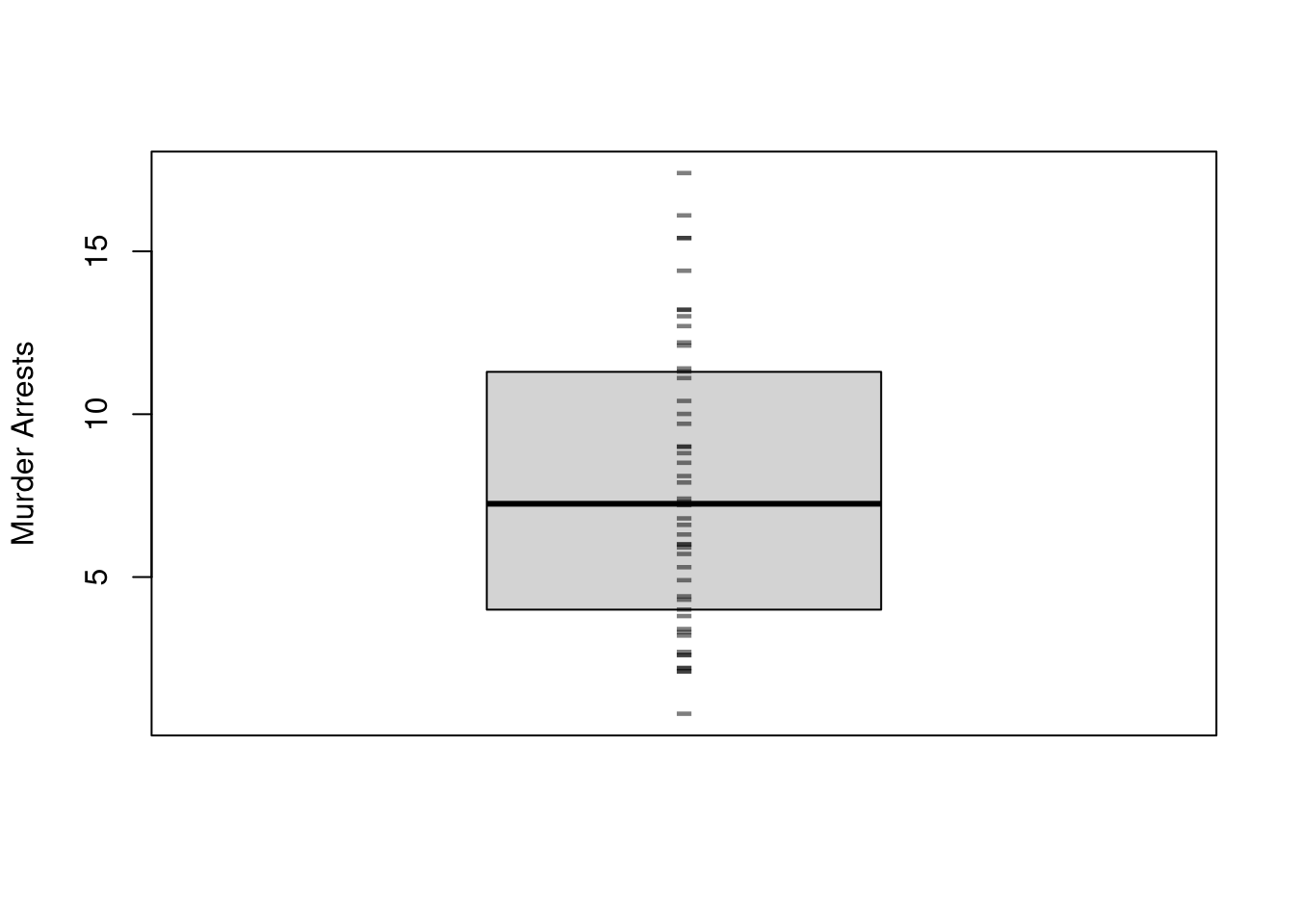
Boxplots also summarize the distribution. The boxplot shows the median (solid black line) and interquartile range (\(IQR=\) upper quartile \(-\) lower quartile; filled box).3 As a default, whiskers are shown as \(1.5\times IQR\) and values beyond that are highlighted as outliers (so whiskers do not typically show the data range). You can alternatively show all the raw data points instead of whisker+outliers.
Code
boxplot(USArrests[,'Murder'],main='', ylab='Murder Arrests',whisklty=0, staplelty=0, outline=F)# Raw Observationsstripchart(USArrests[,'Murder'],pch='-', col=grey(0,.5), cex=2,vert=T, add=T)
We will not cover the statistical analysis of text in this course, but strings are amenable to statistical analysis.↩︎
If \(L\) distinct bins exactly span the range, then \(h=[\text{max}(\hat{X}_{i}) - \text{min}(\hat{X}_{i})]/L\) and \(x\in \left\{ \frac{\ell h}{2} + \text{min}(\hat{X}_{i}) \right\}_{\ell=1}^{L}\).↩︎