8  Misc. Univariate Topics

8.1 Data Transformations

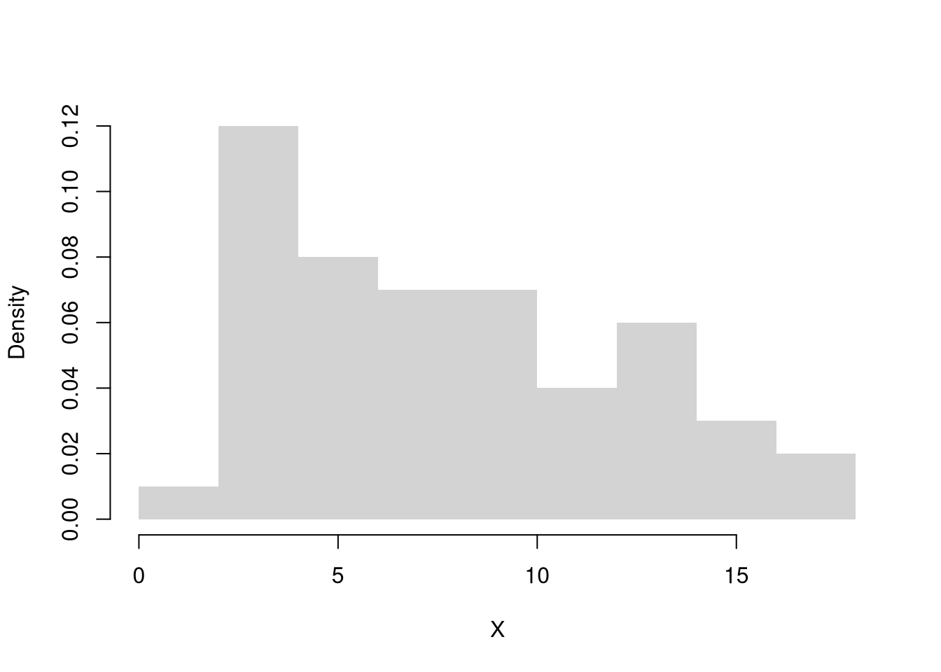
Transformations can stabilize variance, reduce skewness, and make model errors closer to Gaussian.

Perhaps the most common examples are power transformations: \(y= x^\lambda\), which includes \(\sqrt{x}\) and \(x^2\).

Other examples include the exponential transformation: \(y=\exp(x)\) for any \(x\in (-\infty, \infty)\) and logarithmic transformation: \(y=\log(x)\) for any \(x>0\).

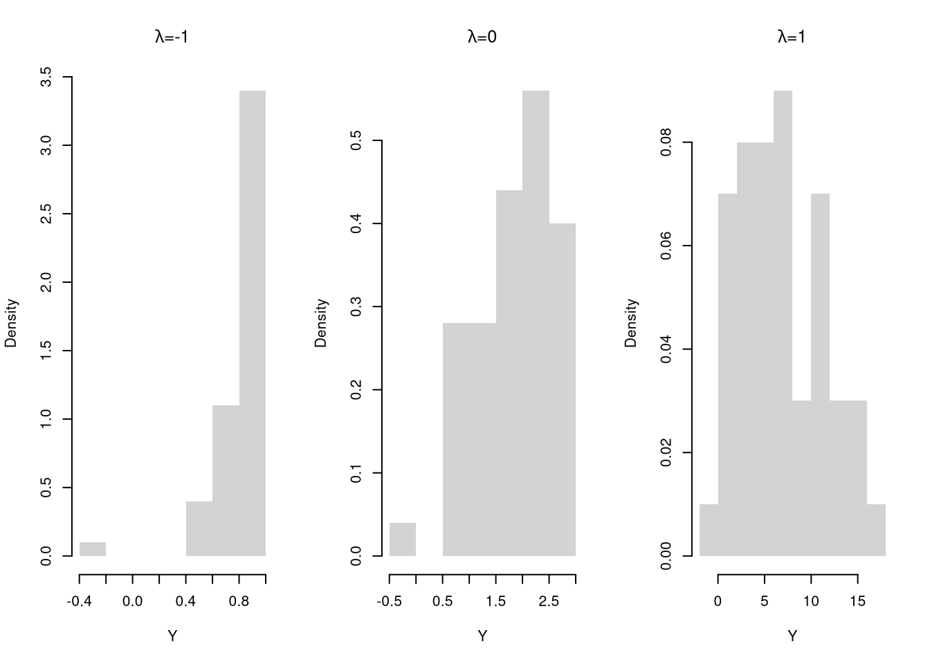
The Box–Cox Transform nests many cases. For \(x>0\) and parameter \(\lambda\), \[\begin{eqnarray} y=\begin{cases} \dfrac{x^\lambda-1}{\lambda}, & \lambda\neq 0,\\ \log\left(x\right) & \lambda=0. \end{cases} \end{eqnarray}\] This function is continuous over \(\lambda\).

# Box–Cox transform and inverse
bc_transform <- function(x, lambda) {
  if (any(x <= 0)) stop("Box-Cox requires x > 0")
  if (abs(lambda) < 1e-8) log(x) else (x^lambda - 1)/lambda
}
bc_inverse <- function(t, lambda) {
  if (abs(lambda) < 1e-8) exp(t) else (lambda*t + 1)^(1/lambda)
}

X <- USArrests$Murder
hist(X, main='', border=NA, freq=F)

par(mfrow=c(1,3))
for(lambda in c(-1,0,1)){
    Y <- bc_transform(X, lambda)
    hist(Y, 
        main=bquote(paste(lambda,'=',.(lambda))),
        border=NA, freq=F)
}

Law of the Unconscious Statistician (LOTUS).

As before, we will represent the random variable as \(X_{i}\), which can take on values \(x\) from the sample space. If \(X_{i}\) is a discrete random variable (a random variable with a discrete sample space) and \(g\) is a function, then \(\mathbb E[g(X)] = \sum_x g(x)Prob(X_{i}=x)\).

Note

Let \(X_{i}\) take values \(\{1,2,3\}\) with \[\begin{eqnarray} Pr(X_{i}=1)=0.2,\quad Prob(X_{i}=2)=0.5,\quad Prob(X_{i}=3)=0.3. \end{eqnarray}\] Let \(g(x)=x^2+1\). Then \(g(1)=1^2+1=2\), \(g(2)=2^2+1=5\), \(g(3)=3^2+1=10\).

Then, by LOTUS, \[\begin{eqnarray} \mathbb E[g(X_{i})]=\sum_x g(x)Prob(X_{i}=x) &=& g(1)\cdot 0.2 + g(2)\cdot 0.5 + g(3)\cdot 0.3 \\ &=& 2 \cdot 0.2 + 5 \cdot 0.5 + 10 \cdot 0.3 \\ &=& 0.4 + 2.5 + 3 = 5.9. \end{eqnarray}\]

x  <- c(1,2,3)
x_probs <- c(0.2,0.5,0.3)
g  <- function(x) x^2 + 1
sum(g(x) * x_probs) 
## [1] 5.9

g  <- function(x) x^2 + 1

# A theoretical example
x <- c(1,2,3,4)
x_probs <- c(1/4, 1/4, 1/4, 1/4)
sum(g(x) * x_probs) 
## [1] 8.5

# A simulation example
X <- sample(x, x_probs, size=1000, replace=T)
mean(g(X))
## [1] 8.543

Tip

If \(X_{i}\) is a continuous random variable (a random variable with a continuous sample space) and \(g\) is a function, then \(\mathbb E[g(X_{i})] = \int_{-\infty}^{\infty} g(x)f(x) dx\).

x <- rexp(5e5, rate = 1)           # X ~ Exp(1)
mean(sqrt(x))                      # LOTUS Simulation
## [1] 0.8868495
sqrt(pi) / 2                       # Exact via LOTUS integral
## [1] 0.8862269

Note that you have already seen the special case where \(g(X_{i})=\left(X_{i}-\mathbb{E}[X_{i}]\right)^2\).

Jensen’s inequality.

Concave functions curve inwards, like the inside of a cave. Convex functions curve outward, the opposite of concave.

If \(g\) is a concave function, then \(g(\mathbb E[X_{i}]) \geq \mathbb E[g(X_{i})]\).

# Continuous Example 1
mean( sqrt(x) )
## [1] 0.8868495
sqrt( mean(x) ) 
## [1] 1.001076

# Continuous Example 2
mean( log(x) )
## [1] -0.5764185
log( mean(x) ) 
## [1] 0.002151259

## Discrete Example
x  <- c(1,2,3)
px <- c(0.2,0.5,0.3)
EX <- sum(x * px)
EX
## [1] 2.1

g  <- sqrt
gEX <- g(EX)
EgX <- sum(g(x) * px)
c(gEX, EgX)
## [1] 1.449138 1.426722

If \(g\) is a convex function, then the inequality reverses: \(g(\mathbb E[X_{i}]) \leq \mathbb E[g(X_{i})]\).

mean( exp(x) )
## [1] 10.06429
exp( mean(x) )  
## [1] 7.389056

8.2 Drawing Samples

To generate a random variable from known distributions, you can use some type of physical machine. E.g., you can roll a fair die to generate Discrete Uniform data or you can roll weighted die to generate Categorical data.

There are also several ways to computationally generate random variables from a probability distribution. Perhaps the most common one is “inverse sampling”. To generate a random variable using inverse sampling, first sample \(p\) from a uniform distribution and then find the associated quantile quantile function \(\widehat{F}^{-1}(p)\).¹

Using Data.

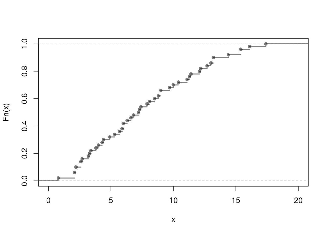
You can generate a random variable from a known empirical distribution. Inverse sampling randomly selects observations from the dataset with equal probabilities. To implement this, we

• order the data and associate each observation with an ECDF value
• draw \(p \in [0,1]\) as a uniform random variable
• find the associated data point on the ECDF

# Empirical Distribution
X <- USArrests$Murder
FX_hat <- ecdf(X)
plot(FX_hat, lwd=2, xlim=c(0,20),
    pch=16, col=grey(0,.5), main='')

# Generating a random variable
p <- runif(3000) ## Multiple Draws
QX_hat <- quantile(X, p, type=1)
QX_hat[1:5]
## 79.64490056% 85.45562837% 72.71574638% 41.93181463% 24.39832431% 
##         12.1         13.0         11.1          6.0          4.0

Using Math.

If you know the distribution function that generates the data, then you can derive the quantile function and do inverse sampling. Here is an in-depth example of the Dagum distribution. The distribution function is \(F(x)=(1+(x/b)^{-a})^{-c}\). For a given probability \(p\), we can then solve for the quantile as \(F^{-1}(p)=\frac{ b p^{\frac{1}{ac}} }{(1-p^{1/c})^{1/a}}\). Afterwhich, we sample \(p\) from a uniform distribution and then find the associated quantile.

# Theoretical Quantile Function (from VGAM::qdagum)
qdagum <- function(p, scale.b=1, shape1.a, shape2.c) {
  # Quantile function (theoretically derived from the CDF)
  ans <- scale.b * (expm1(-log(p) / shape2.c))^(-1 / shape1.a)
  # Special known cases
  ans[p == 0] <- 0
  ans[p == 1] <- Inf
  # Safety Checks
  ans[p < 0] <- NaN
  ans[p > 1] <- NaN
  if(scale.b <= 0 | shape1.a <= 0 | shape2.c <= 0){ ans <- ans*NaN }
  # Return
  return(ans)
}

# Generate Random Variables (VGAM::rdagum)
rdagum <-function(n, scale.b=1, shape1.a, shape2.c){
    p <- runif(n) # generate random probabilities
    x <- qdagum(p, scale.b=scale.b, shape1.a=shape1.a, shape2.c=shape2.c) #find the inverses
    return(x)
}

# Example
set.seed(123)
X <- rdagum(3000,1,3,1)
X[1:5]
## [1] 0.7390476 1.5499868 0.8845006 1.9616251 2.5091656

8.3 Set Theory

Let the sample space contain events \(A\) and \(B\), with their probability denoted as \(Prob(A)\) and \(Prob(B)\). Then

• the union: \(A\cup B\), refers to either event occurring
• the intersection: \(A\cap B\), refers to both events occurring
• the events \(A\) and \(B\) are mutually exclusive if and only if \(A\cap B\) is empty.
• the inclusion–exclusion rule is: \(Prob(A\cup B)=Prob(A)+Prob(B)-Prob(A\cap B)\).
• the events \(A\) and \(B\) are mutually independent if and only if \(Prob(A\cap B)=Prob(A) Prob(B)\).
• the conditional probability is \(Prob(A \mid B) = Prob(A \cap B)/ P(B)\).

For example, consider a six sided die where

• \(A\): number \(>\!2\), which implies \(A=\{3,4,5,6\}\)
• \(B\): number is even, which implies \(B=\{2,4,6\}\)
• To check mutually exclusive: notice \(A\cap B=\{4,6\}\) which is not empty. So No, event \(A\) and event \(B\) are not mutually exclusive.

Further assuming the die are fair

• \(Prob(A)=4/6=2/3\) and \(Prob(B)=3/6=1/2\)
• \(A\cup B=\{2,3,4,5,6\}\), which implies \(Prob(A\cup B)=5/6\).
• \(A\cap B=\{4,6\}\), which implies \(Prob(A\cap B)=2/6=1/3\).
• To check independence: notice \(Prob(A\cap B)=1/3 = (2/3) (1/2) = Prob(A)Prob(B)\). So Yes, event \(A\) and event \(B\) are mutually independent.
• Finally, the conditional probability of \(Prob(\text{die is} >2 \mid \text{die shows an even number}) = Prob(A \mid B) = Prob(A \cap B)/ P(B) = \frac{1/3}{2/3}=2/3\).

# Simulation verification
set.seed(123)
rolls <- sample(1:6, 1e6, replace = TRUE)
A <- rolls > 2
B <- rolls %% 2 == 0
P_AcondB <- mean(A & B) / mean(B)
round(P_AcondB, 3)
## [1] 0.667

Tip

Consider a six sided die with sample space \(\{1,2,3,4,5,6\}\) where each outcome is each equally likely. What is \(Prob(\text{die is odd or }<5)\)? Denote the odd events as \(A=\{1,3,5\}\) and the less than five events as \(B=\{1,2,3,4\}\). Then

• \(A\cup B=\{1,3\}\), which implies \(Prob(A\cap B)=2/6=1/3\).
• \(Prob(A)=3/6=1/2\) and \(Prob(B)=4/6=2/3\).
• By inclusion–exclusion: \(Prob(A\cup B)=Prob(A)+Prob(B)-Prob(A\cap B)=1/2+2/3-1/3=5/6\).

Now find \(Prob(\text{die is even and }<5)\). Verify your answer with a computer simulation.

8.4 Count Distributions

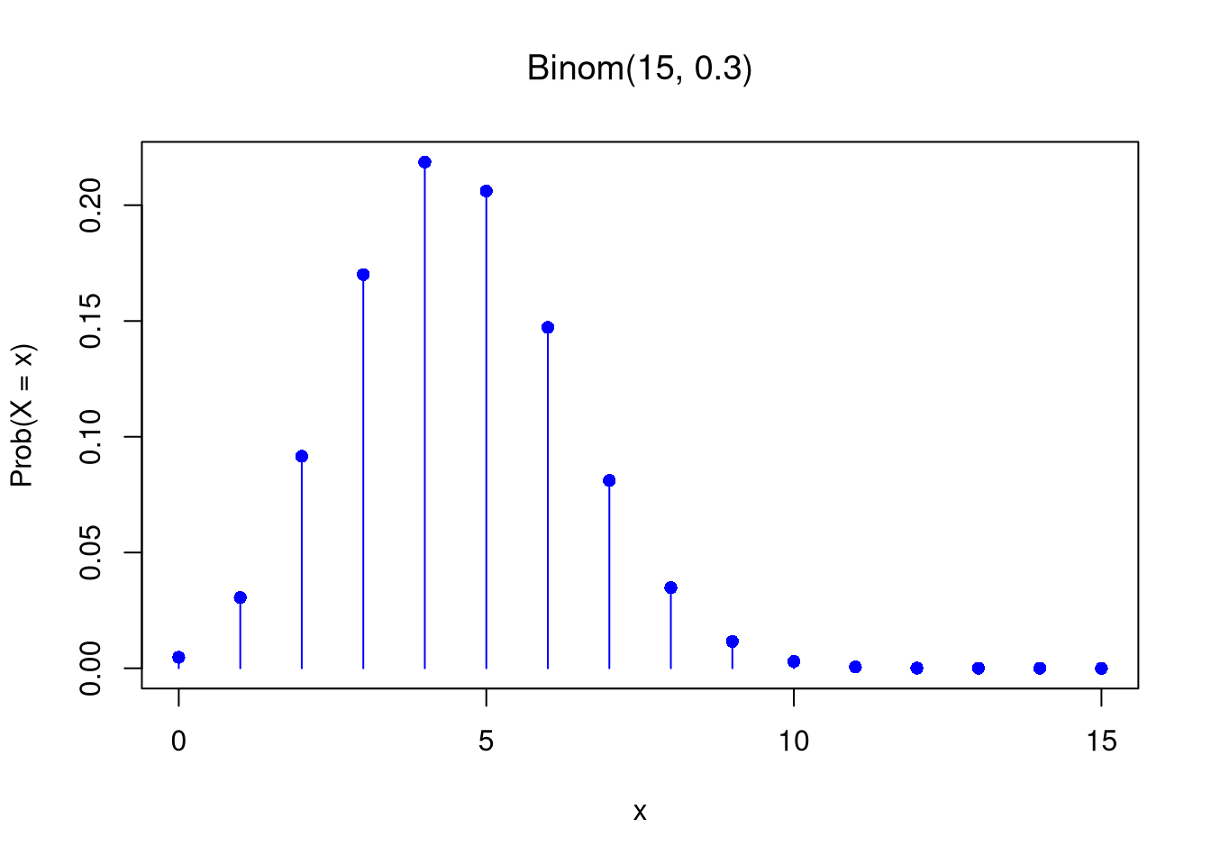
Binomial.

The sum of \(n\) Bernoulli trials (number of successes)

• Discrete, support \(\{0,1,\ldots,n\}\)
• Probability Mass Function: \(Prob(X_{i}=x)=\binom{n}{x}p^k(1-p)^{n-x}\)
• See https://en.wikipedia.org/wiki/Binomial_distribution
• A common use case: How many heads will I get when I flip a coin twice?

## Minimal example
n <- 15
p <- 0.3

# PMF plot
x <- 0:n
f_x <- dbinom(x, n, p)
plot(x, f_x, type = "h", col = "blue",
    main='',  xlab = "x", ylab = "Prob(X = x)")
title(bquote(paste('Binom(',.(n),', ',.(p), ')' ) ))
points(x, f_x, pch = 16, col = "blue")

# Simulate:  Compare empirical vs theoretical
#X <- rbinom(1e4, size = n, prob = p)
#c(emp_mean = mean(X), th_mean = n*p)
#c(emp_var  = var(X),  th_var  = n*p*(1-p))

Tip

Suppose that employees at a company are \(70%\) female and \(30%\) male. If we select a random sample of eight employees, what is the probability that more than \(2\) in the sample are female?

Tip

Show that \(\mathbb{E}[X_{i}]=np\) and \(\mathbb{V}[X_{i}]=np(1-p)\).

The Binomial Limit Theorem (de Moivre–Laplace theorem) says that as \(n\) grows large, with \(p \in (0,1)\) staying fixed, the Binomial distribution is approximately normal with mean \(np\) and variance \(np(1-p)\)

Tip

The unemployment rate is \(10%\). Suppose that \(100\) employable people are selected randomly. What is the probability that this sample contains between \(9\) and \(12\) unemployed people. Use the normal approximation to binomial probabilities (parameters \(\mu=100, \sigma=9.49\)).

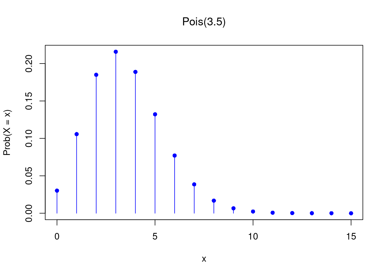
Poisson.

The number of events in a fixed interval

• Discrete, support \(\{0,1,2,\ldots\}\)
• Probability Mass Function: \(Prob(X_{i}=x)=e^{-\lambda}\lambda^x/x!\)
• See https://en.wikipedia.org/wiki/Poisson_distribution
• A common use case: How many cars will show up in the lot tomorrow?

## Minimal example
lambda <- 3.5

# PMF plot
x <- 0:15
f_x <- dpois(x, lambda)
plot(x, f_x, type="h", col="blue",
     xlab = "x", ylab = "Prob(X = x)")
points(x, f_x, pch = 16, col = "blue")
title(bquote(paste('Pois(',.(lambda), ')')))

# Simulate: Compare empirical vs theoretical
#X <- rpois(1e4, lambda)
#c(emp_mean = mean(X), th_mean = lambda)
#c(emp_var  = var(X),  th_var  = lambda)

Tip

Show that \(\mathbb{E}[X_{i}] = \mathbb{V}[X_{i}]= \lambda\).

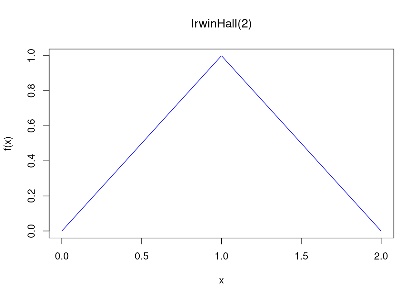
Irwin–Hall.

The sum of \(n\) i.i.d. \(\text{Uniform}(0,1)\).

• Continuous, support \([0,n]\)
• Probability Density Function: \(f(x) = \dfrac{1}{(n-1)!} \displaystyle\sum_{k=0}^{\lfloor x \rfloor} (-1)^k \binom{n}{k} (x - k)^{n-1}\) for \(x \in [0,n]\), and \(0\) otherwise
• See https://en.wikipedia.org/wiki/Irwin%E2%80%93Hall_distribution
• A common use case: representing the sum of many small independent financial shocks

## Minimal example (base R)
# Irwin–Hall PDF function
dirwinhall <- function(x, n) {
    f_x <- vector(length=length(x))
    for(i in seq(x)) {
        xx <- x[i]
        if(xx < 0 | xx > n){
            f_x[i] <- 0 
        } else {
            k <- 0:floor(xx)
            f_k <- sum((-1)^k*choose(n, k)*(xx-k)^(n-1))/factorial(n-1)
            f_x[i] <- f_k
        }}
    return(f_x)
}

# Parameters
n <- 2
x <- seq(0, n, length.out = 500)

# Compute and plot PDF
f_x <- dirwinhall(x, n)
plot(x, f_x, type="l", col="blue",
    main='', xlab = "x", ylab = "f(x)")
title(bquote(paste('IrwinHall(',.(n), ')')))

See also the Bates Distribution.

8.5 Beyond Basic Programming

Use expansion “packages” for more functionality.

Most packages can be easily installed, and you only need to install packages once.

# common packages for tables/figures
install.packages("plotly")
install.packages("reactable")
install.packages("stargazer")

# common packages for data/teaching
install.packages("AER")
install.packages("Ecdat")
install.packages('wooldridge')

# other packages for statistics and data handling
install.packages("extraDistr")
install.packages("twosamples")
install.packages("data.table")

You need to load the package via library every time you want the extended functionality. For example, to generate exotic probability distributions

library(extraDistr)

par(mfrow=c(1,2))
for(p in c(-.5,0)){
    x <- rgev(2000, mu=0, sigma=1, xi=p)
    hist(x, breaks=50, border=NA, main=NA, freq=F)
}
title('GEV densities', outer=T, line=-1)

library(extraDistr)

par(mfrow=c(1,3))
for(p in c(-1, 0,2)){
    x <- rtlambda(2000, p)
    hist(x, breaks=100, border=NA, main=NA, freq=F)
}
title('Tukey-Lambda densities', outer=T, line=-1)

The most common tasks also have cheatsheets you can use.

Updating.

Make sure R and your packages are up to date. The current version of R and any packages used can be found (and recorded) with

sessionInfo()

To update your R packages, use

update.packages()

Base.

While additional packages can make your code faster, they also create dependancies that can lead to problems. So learn base R well before becoming dependent on other packages

• https://bitsofanalytics.org/posts/base-vs-tidy/
• https://jtr13.github.io/cc21fall2/comparison-among-base-r-tidyverse-and-datatable.html

Advanced Programming.

Advanced and Optional

Sometimes you will want to install a package from GitHub. For this, you can use devtools or its light-weight version remotes

install.packages("devtools")
install.packages("remotes")

Note that to install devtools, you also need to have developer tools installed on your computer.

• Windows: Rtools
• Mac: Xcode

To color terminal output on Linux systems, you can use the colorout package

library(remotes)
# Install <https://github.com/jalvesaq/colorout
# to .libPaths()[1]
install_github('jalvesaq/colorout')
library(colorout)

Note that after updating R, you can update all packages stored in all .libPaths() with the following command

update.packages(checkBuilt=T, ask=F)
# install.packages(old.packages(checkBuilt=T)[,"Package"])

Sometimes there is a problem. To find specific broken packages after an update

library(purrr)

set_names(.libPaths()) %>%
  map(function(lib) {
    .packages(all.available = TRUE, lib.loc = lib) %>%
        keep(function(pkg) {
            f <- system.file('Meta', 'package.rds', package = pkg, lib.loc = lib)
            tryCatch({readRDS(f); FALSE}, error = function(e) TRUE)
        })
  })
# https://stackoverflow.com/questions/31935516/installing-r-packages-error-in-readrdsfile-error-reading-from-connection/55997765

To remove packages duplicated in multiple libraries

# Libraries
i <- installed.packages()
libs <- .libPaths()
# Find Duplicated Packages
i1 <- i[ i[,'LibPath']==libs[1], ]
i2 <- i[ i[,'LibPath']==libs[2], ]
dups <- i2[,'Package'] %in% i1[,'Package']
all( dups )
# Remove
remove.packages(  i2[,'Package'], libs[2] )

---

1. Drawing random uniform samples with computers is actually quite complex and beyond the scope of this course.