Code
#All possible samples of two from {1,2,3,4}
#{1,2} {1,3}, {3,4}
#{2,3} {2,4}
#{3,4}
choose(4,2)
## [1] 6

# Simple random sample (no duplicates, equal probability)
x <- c(1,2,3,4)
sample(x, 2, replace=F)
## [1] 4 2A sample is a subset of the population. A simple random sample is a sample where each possible sample of size n has the same probability of being selected.
#All possible samples of two from {1,2,3,4}
#{1,2} {1,3}, {3,4}
#{2,3} {2,4}
#{3,4}
choose(4,2)
## [1] 6
# Simple random sample (no duplicates, equal probability)
x <- c(1,2,3,4)
sample(x, 2, replace=F)
## [1] 4 2Often, we think of the population as being infinitely large. This is an approximation that makes mathematical and computational work much simpler.
#All possible samples of two from an enormous bag of numbers {1,2,3,4}
#{1,1} {1,2} {1,3}, {3,4}
#{2,2} {2,3} {2,4}
#{3,3} {3,4}
#{4,4}

# Simple random sample (duplicates, equal probability)
sample(x, 2, replace=T)
## [1] 1 3
Intuition for infinite populations: imagine drawing names from a giant urn. If the urn has only \(10\) names, then removing one name slightly changes the composition of the urn, and the probabilities shift for the next name you draw. Now imagine the urn has \(100\) billion names, so that removing one makes no noticeable difference. We can pretend the composition never changes: each draw is essentially identical and independent (iid). We can actually guarantee the names are iid by putting any names drawn back into the urn (sampling with replacement).
The sampling distribution of a statistic shows us how much a statistic varies from sample to sample.
For example, the sampling distribution of the mean shows how the sample mean varies from sample to sample to sample. The sampling distribution of mean can also be referred to as the probability distribution of the sample mean.
Given ages for population of \(4\) students, compute the sampling distribution for the mean with samples of \(n=2\).
X <- c(18,20,22,24) # Ages for student population
# six possible samples
m1 <- mean( X[c(1,2)] ) #{1,2}
m2 <- mean( X[c(1,3)] ) #{1,3}
m3 <- mean( X[c(1,4)] ) #{3,4}
m4 <- mean( X[c(2,3)] ) #{2,3}
m5 <- mean( X[c(2,4)] ) #{2,4}
m6 <- mean( X[c(3,4)] ) #{3,4}
# sampling distribution
sample_means <- c(m1, m2, m3, m4, m5, m6)
hist(sample_means,
    freq=F, breaks=100,
    main='', border=F)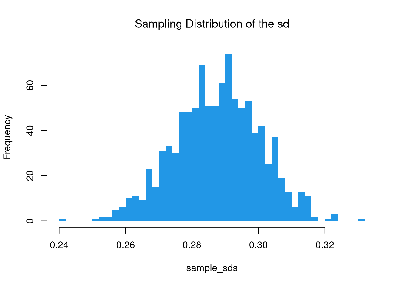
Now compute the sampling distribution for the median with samples of \(n=3\).
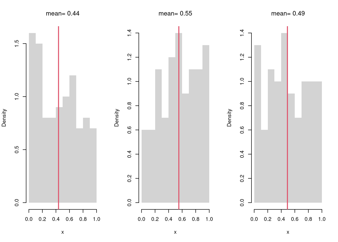
# Three Sample Example w/ Visual
par(mfrow=c(1,3))
for(b in 1:3){
    x <- runif(100)
    m <-  mean(x)
    hist(x,
        breaks=seq(0,1,by=.1), #for comparability
        freq=F, main=NA, border=NA)
    abline(v=m, col=2, lwd=2)
    title(paste0('mean= ', round(m,2)),  font.main=1)
}
Examine the sampling distribution of the mean
# Many sample example
sample_means <- vector(length=500)
for(i in seq_along(sample_means)){
    x <- runif(1000)
    m <- mean(x)
    sample_means[i] <- m
}
hist(sample_means,
    breaks=seq(0.45,0.55,by=.001),
    border=NA, freq=F,
    col=2, font.main=1,
    xlab=expression(hat(M)),
    main='Sampling Distribution of the mean')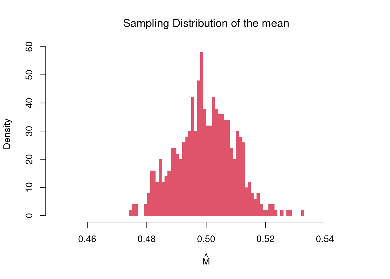
In this figure, you see two the most profound results known in statistics
There are different variants of the Law of Large Numbers (LLN), but they all say some version of “the sample mean is centered around the true mean, and more tightly centered with more data”.
Notice where the sampling distribution is centered
m_LLLN <- mean(sample_means)
round(m_LLLN, 3)
## [1] 0.5
and more tightly centered with more data
par(mfrow=c(1,3))
for(n in c(5,50,500)){
    sample_means_n <- vector(length=299)
    for(i in seq_along(sample_means_n)){
        x <- runif(n)
        m <- mean(x)
        sample_means_n[i] <- m
    }
    hist(sample_means_n,
        breaks=seq(0,1,by=.01),
        border=NA, freq=F,
        col=2, font.main=1,
        xlab=expression(hat(M)),
        main=paste0('n=',n) )
}
Plot the variability of the sample mean as a function of sample size
n_seq <- seq(1, 40)
sd_seq <- vector(length=length(n_seq))
for(n in seq_along(sd_seq)){
    sample_means_n <- vector(length=499)
    for(i in seq_along(sample_means_n)){
        x <- runif(n)
        m <- mean(x)
        sample_means_n[i] <- m
    }
    sd_seq[n] <- sd(sample_means_n)
}
plot(n_seq, sd_seq, pch=16, col=grey(0,0.5),
    xlab='n', ylab='sd of sample means', main='')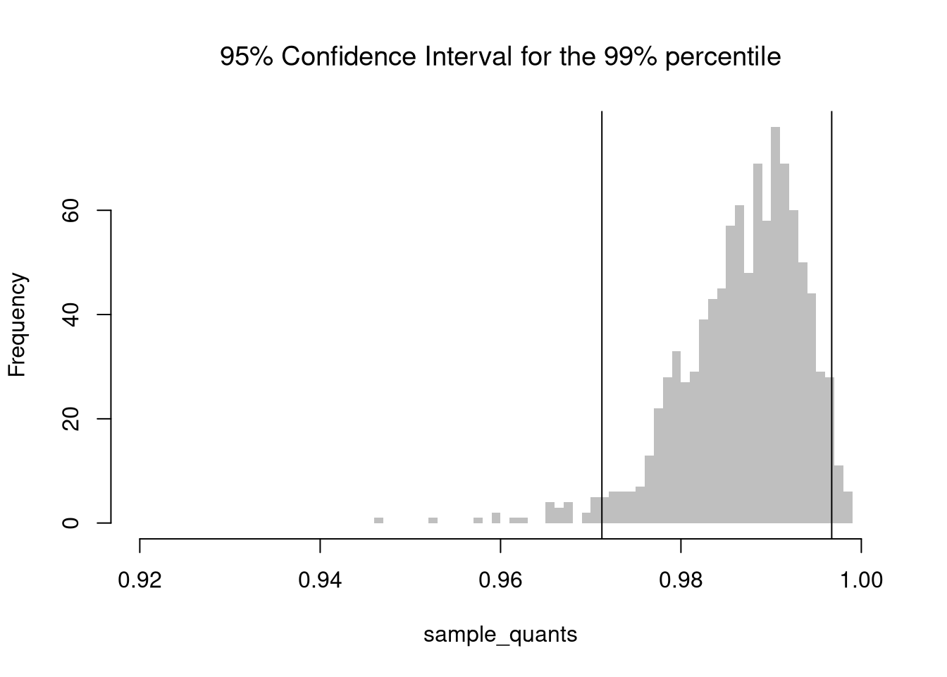
The Law of Large Numbers generalizes to many other statistics, like median or sd. When a statistic converges in probability to the quantity they are meant to estimate, they are called consistent.
par(mfrow=c(1,3))
for(n in c(5,50,500)){
    sample_quants_n <- vector(length=299)
    for(i in seq_along(sample_quants_n)){
        x <- runif(n)
        m <- quantile(x, probs=0.75) #upper quartile
        sample_quants_n[i] <- m
    }
    hist(sample_quants_n,
        breaks=seq(0,1,by=.01),
        border=NA, freq=F,
        col=2, font.main=1,
        xlab="Sample Quantile",
        main=paste0('n=',n) )
}
There are different variants of the central limit theorem (CLT), but they all say some version of “the sampling distribution of a statistic is approximately normal”. For example, the sampling distribution of the mean, shown above, is approximately normal.
hist(sample_means,
    breaks=seq(0.45,0.55,by=.001),
    border=NA, freq=F,
    col=2, font.main=1,
    xlab=expression(hat(M)),
    main='Sampling Distribution of the mean')

## Approximately normal?
mu <- mean(sample_means)
mu_sd <- sd(sample_means)
x <- seq(0.1, 0.9, by=0.001)
fx <- dnorm(x, mu, mu_sd)
lines(x, fx, col='red')
For an example with another statistic, let’s the sampling distribution of the standard deviation.
# CLT example of the "sd" statistic
sample_sds <- vector(length=1000)
for(i in seq_along(sample_sds)){
    x <- runif(100) # same distribution
    s <- sd(x) # different statistic
    sample_sds[i] <- s
}
hist(sample_sds,
    breaks=seq(0.2,0.4,by=.01),
    border=NA, freq=F,
    col=4, font.main=1,
    xlab=expression(hat(S)),
    main='Sampling Distribution of the sd')

## Approximately normal?
mu <- mean(sample_sds)
mu_sd <- sd(sample_sds)
x <- seq(0.1, 0.9, by=0.001)
fx <- dnorm(x, mu, mu_sd)
lines(x, fx, col='blue')
# Try another function, such as
my_function <- function(x){ diff(range(exp(x))) }

# try another random variable, such as rexp(100) instead of runif(100)
It is beyond this class to prove this result mathematically, but you should know that not all sampling distributions are standard normal. The CLT approximation is better for “large \(n\)” datasets with “well behaved” variances. The CLT also does not apply to “extreme” statistics.
For example of “extreme” statistics, examine the sampling distribution of min and max statistics.
# Create 300 samples, each with 1000 random uniform variables
x_samples <- matrix(nrow=300, ncol=1000)
for(i in seq(1,nrow(x_samples))){
    x_samples[i,] <- runif(1000)
}
# Each row is a new sample
length(x_samples[1,])
## [1] 1000

# Compute min and max for each sample
x_mins <- apply(x_samples, 1, quantile, probs=0)
x_maxs <- apply(x_samples, 1, quantile, probs=1)

# Plot the sampling distributions of min, median, and max
# Median looks normal. Maximum and Minumum do not!
par(mfrow=c(1,2))
hist(x_mins, breaks=100, main='Min', font.main=1,
    xlab=expression(hat(Q)[0]), border=NA, freq=F)
hist(x_maxs, breaks=100, main='Max', font.main=1,
    xlab=expression(hat(Q)[1]), border=NA, freq=F)
title('Sampling Distributions', outer=T, line=-1, adj=0)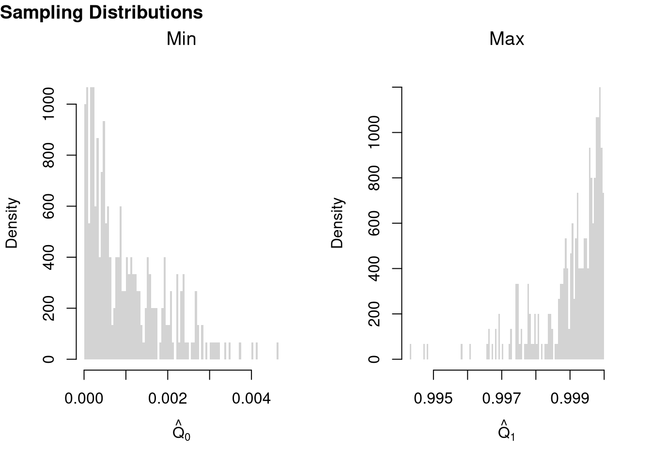
Often, we only have one sample. How then can we estimate the sampling distribution of a statistic?
sample_dat <- USArrests[,'Murder']
sample_mean <- mean(sample_dat)
sample_mean
## [1] 7.788
We can “resample” our data. Hesterberg (2015) provides a nice illustration of the idea. The two most basic versions are the jackknife and the bootstrap, which are discussed below.
Note that we do not use the mean of the resampled statistics as a replacement for the original estimate. This is because the resampled distributions are centered at the observed statistic, not the population parameter. (The bootstrapped mean is centered at the sample mean, for example, not the population mean.) This means that we cannot use resampling to improve on \(\hat{M}\). We use resampling to estimate sampling variability.
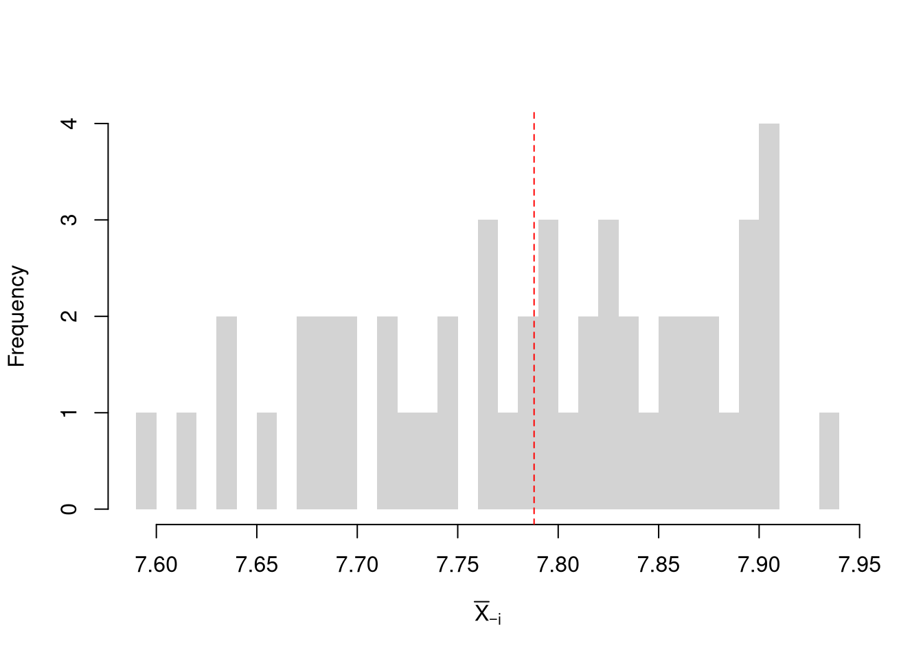
Here, we compute all “leave-one-out” estimates. Specifically, for a dataset with \(n\) observations, the jackknife uses \(n-1\) observations other than \(i\) for each unique subsample.
sample_dat <- USArrests[,'Murder']
sample_mean <- mean(sample_dat)

# Jackknife Estimates
n <- length(sample_dat)
jackknife_means <- vector(length=n)
for(i in seq_along(jackknife_means)){
    dat_noti <- sample_dat[-i]
    mean_noti <- mean(dat_noti)
    jackknife_means[i] <- mean_noti
}
hist(jackknife_means, breaks=25,
    border=NA, freq=F,
    main='', xlab=expression(hat(M)[-i]))
abline(v=sample_mean, col='red', lty=2)
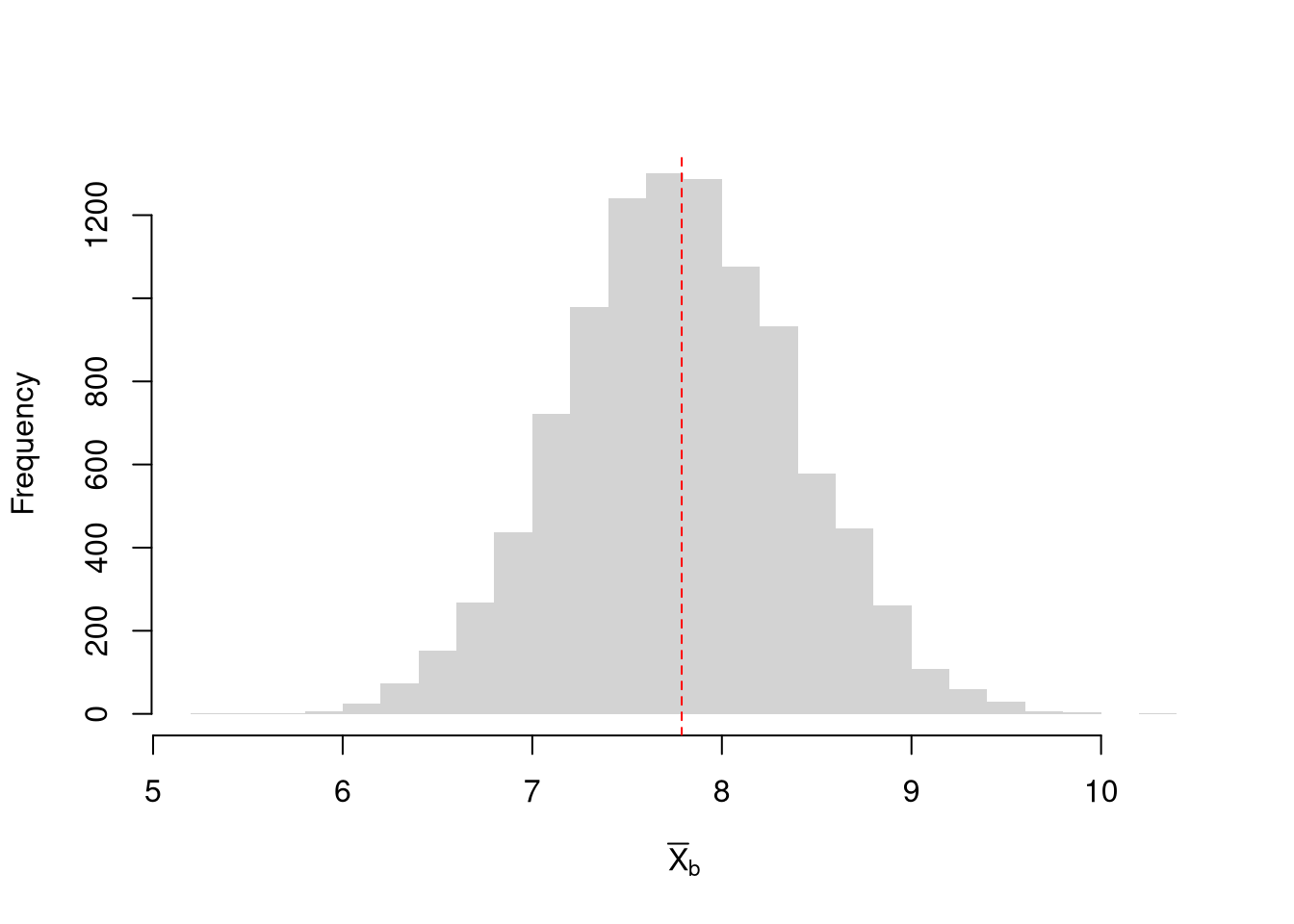
Here, we draw \(n\) observations with replacement from the original data to create a bootstrap sample and calculate a statistic. Each bootstrap sample \(b=1...B\) uses a random subset of observations to compute a statistic. We repeat that many times, say \(B=9999\), to estimate the sampling distribution.
# Bootstrap estimates
bootstrap_means <- vector(length=9999)
for(b in seq_along(bootstrap_means)){
    dat_id <- seq(1,n)
    boot_id <- sample(dat_id , replace=T)
    dat_b  <- sample_dat[boot_id] # c.f. jackknife
    mean_b <- mean(dat_b)
    bootstrap_means[b] <-mean_b
}

hist(bootstrap_means, breaks=25,
    border=NA, freq=F,
    main='', xlab=expression(hat(M)[b]))
abline(v=sample_mean, col='red', lty=2)
Why does this work? The sample: \(\{\hat{X}_{1}, \hat{X}_{2}, ... \hat{X}_{n}\}\) is drawn from a CDF \(F\). Each bootstrap sample: \(\{\hat{X}_{1}^{(b)}, \hat{X}_{2}^{(b)}, ... \hat{X}_{n}^{(b)}\}\) is drawn from the ECDF \(\hat{F}\). With \(\hat{F} \approx F\), each bootstrap sample is approximately a random sample. So when we compute a statistic on each bootstrap sample, we approximate the sampling distribution of the statistic.
Using either the bootstrap or jackknife distribution, we can estimate variability via the Standard Error: the standard deviation of your statistic across different samples (square rooted). In either case, this differs from the standard deviation of the data within your sample.
sd(sample_dat) # standard deviation
## [1] 4.35551
sd(bootstrap_means) # standard error
## [1] 0.6040716
Also note that each additional data point you have provides more information, which ultimately decreases the standard error of your estimates. This is why statisticians will often recommend that you to get more data. However, the improvement in the standard error increases at a diminishing rate. In economics, this is known as diminishing returns and why economists may recommend you do not get more data.
B <- 1000 # number of bootstrap samples
Nseq <- seq(1,100, by=1) # different sample sizes

SE <- vector(length=length(Nseq))
for(n in Nseq){
    sample_statistics_n <- vector(length=B)
    for(b in seq(1,B)){
        x_b <- rnorm(n) # Sample of size n
        x_stat_b <- quantile(x_b, probs=.4) # Stat of interest
        sample_statistics_n[b] <- x_stat_b
    }
    se_n <- sd(sample_statistics_n) # How much the stat varies across samples
    SE[n] <- se_n
}

plot(Nseq, SE, pch=16, col=grey(0,.5),
    ylab='standard error', xlab='sample size')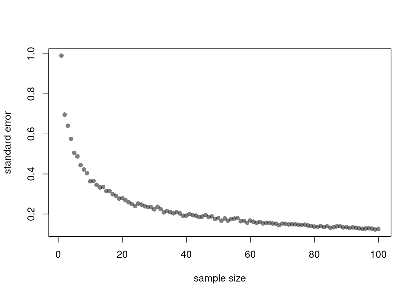
The LLN follows from a famous theoretical result in statistics, Linearity of Expectations: the expected value of a sum of random variables equals the sum of their individual expected values. To be concrete, suppose we take \(n\) random variables, each one denoted as \(X_{i}\). Then, for constants \(a,b,1/n\), we have \[\begin{eqnarray} \mathbb{E}[a X_{1}+ b X_{2}] &=& a \mathbb{E}[X_{1}]+ b \mathbb{E}[X_{2}]\\ \mathbb{E}\left[M\right] &=& \mathbb{E}\left[ \sum_{i=1}^{n} X_{i}/n \right] = \sum_{i=1}^{n} \mathbb{E}[X_{i}]/n \end{eqnarray}\] Assuming each data point has identical means; \(\mathbb{E}[X_{i}]=\mu\), the expected value of the sample average is the mean; \(\mathbb{E}\left[M\right] = \sum_{i=1}^{n} \mu/n = \mu\).
Note that the estimator \(M\) differs from the particular estimate you calculated for your sample, \(\hat{M}\). For example, consider flipping a coin three times: \(M\) corresponds to a theoretical value before you flip the coins and \(\hat{M}\) corresponds to a specific value after you flip the coins.
Another famous theoretical result in statistics is that if we have independent and identical data (i.e., that each random variable \(X_{i}\) has the same mean \(\mu\), same variance \(\sigma^2\), and is drawn without any dependence on the previous draws), then the standard error of the sample mean is “root n” proportional to the theoretical standard error. Intuitively, this follows from thinking of the variance as a type of mean (the mean squared deviation from \(\mu\)). \[\begin{eqnarray} \mathbb{V}\left( M \right) &=& \mathbb{V}\left( \frac{\sum_{i}^{n} X_{i}}{n} \right) = \sum_{i}^{n} \mathbb{V}\left(\frac{X_{i}}{n}\right) = \sum_{i}^{n} \frac{\sigma^2}{n^2} = \sigma^2/n\\ \mathbb{s}\left(M\right) &=& \sqrt{\mathbb{V}\left( M \right) } = \sqrt{\sigma^2/n} = \sigma/\sqrt{n}. \end{eqnarray}\]
Note that the standard deviation refers to variance within a single sample, and is hence different from the standard error. Nonetheless, it can be used to estimate the variability of the mean: we can estimate \(\mathbb{s}\left(M\right)\) with \(\hat{S}/\sqrt{n}\), where \(\hat{S}\) is the standard deviation of the sample. This estimate is often a little different from than the bootstrap estimate, as it is based on idealistic theoretical assumptions whereas the bootstrap estimate is driven by data that are often not ideal.
boot_se <- sd(bootstrap_means)

theory_se <- sd(sample_dat)/sqrt(n)

c(boot_se, theory_se)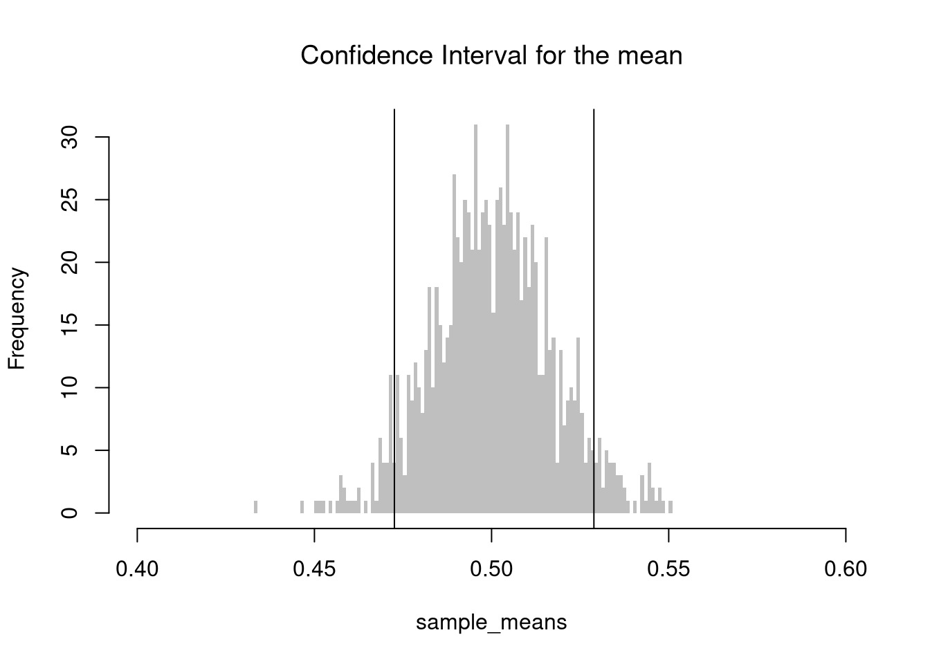
## [1] 0.6040716 0.4355510Sometimes, the sampling distribution is approximately normal (according to the CLT). In this case, you can use a standard error and the normal distribution to get a confidence interval.
# Standard Errors
theory_sd <- sd(sample_dat1)/sqrt(length(sample_dat1))
## Normal CI
theory_quantile <- qnorm(c(0.025, 0.975))
theory_ci <- mean(sample_dat1) + theory_quantile*theory_sd

# compare with: boot_ci, jack_ciSee