Code
# Bivariate Data from USArrests
xy <- USArrests[,c('Murder','UrbanPop')]
xy[1,]
##         Murder UrbanPop
## Alabama 13.2 58We will now study them in more detail. Suppose we have two discrete variables \(X_{i}\) and \(Y_{i}\). The data for each observation data can be grouped together as a vector \((X_{i}, Y_{i})\).
# Bivariate Data from USArrests
xy <- USArrests[,c('Murder','UrbanPop')]
xy[1,]
## Murder UrbanPop
## Alabama 13.2 58Scatterplots are used frequently to summarize the joint relationship between two variables, multiple observations of \((X_{i}, Y_{i})\). They can be enhanced in several ways. As a default, use semi-transparent points so as not to hide any points (and perhaps see if your observations are concentrated anywhere). You can also add other features that help summarize the relationship, although I will defer this until later.
plot(Murder~UrbanPop, USArrests, pch=16, col=grey(0.,.5))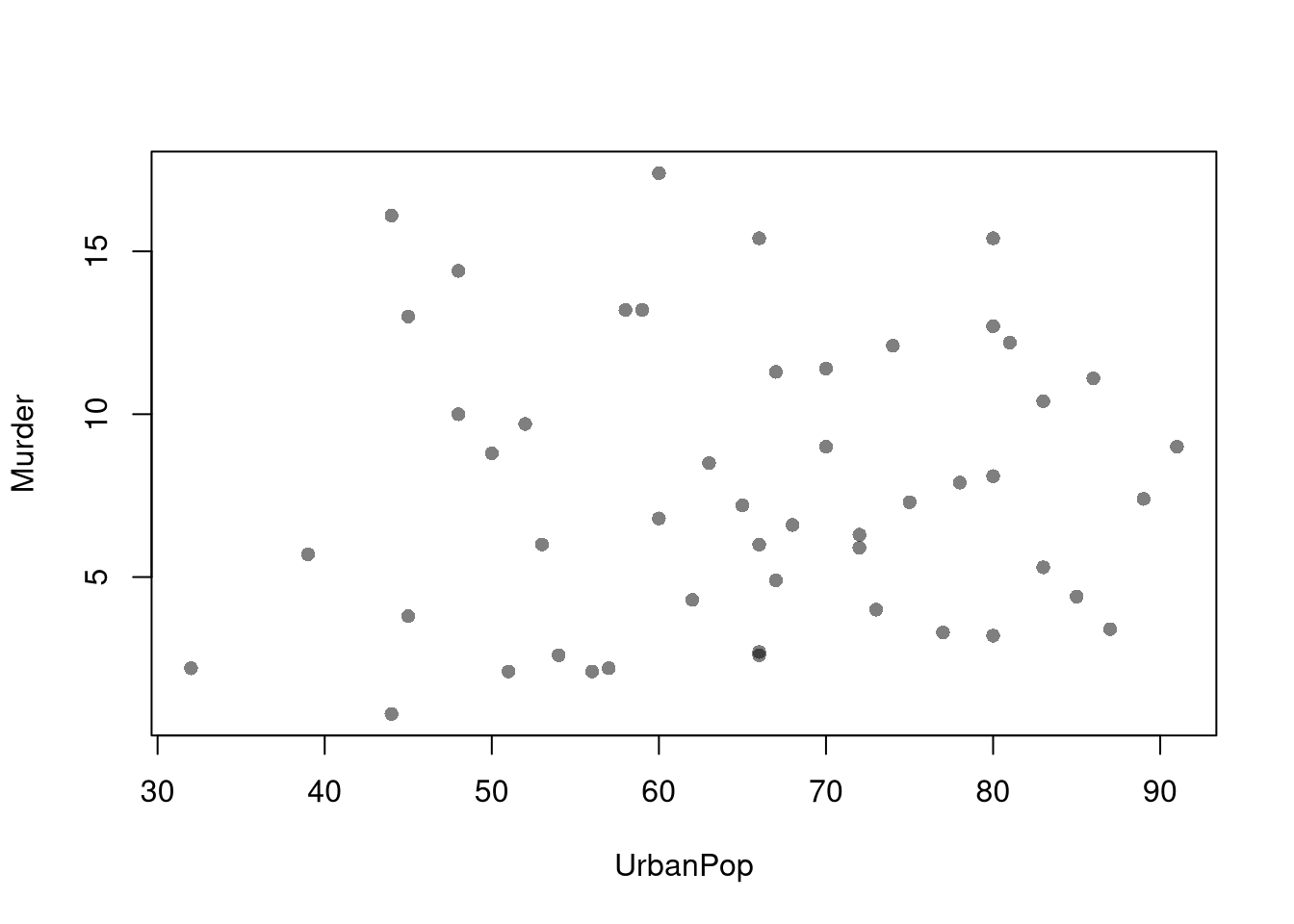
If you have many points, you can also use a 2D histogram instead. https://plotly.com/r/2D-Histogram/.
library(plotly)
fig <- plot_ly(
    USArrests, x = ~UrbanPop, y = ~Assault)
fig <- add_histogram2d(fig, nbinsx=25, nbinsy=25)
figYou can also show the distributions of each variable along each axis.
# Setup Plot
layout( matrix(c(2,0,1,3), ncol=2, byrow=TRUE),
    widths=c(9/10,1/10), heights=c(1/10,9/10))

# Scatterplot
par(mar=c(4,4,1,1))
plot(Murder~UrbanPop, USArrests, pch=16, col=rgb(0,0,0,.5))

# Add Marginals
par(mar=c(0,4,1,1))
xhist <- hist(USArrests[,'UrbanPop'], plot=FALSE)
barplot(xhist[['counts']], axes=FALSE, space=0, border=NA)

par(mar=c(4,0,1,1))
yhist <- hist(USArrests[,'Murder'], plot=FALSE)
barplot(yhist[['counts']], axes=FALSE, space=0, horiz=TRUE, border=NA)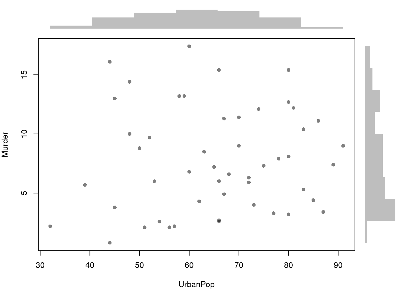
We can show how distributions and densities change according to a second (or even third) variable using data splits. E.g.,
# Tailored Histogram
ylim <- c(0,8)
xbks <-  seq(min(USArrests[,'Murder'])-1, max(USArrests[,'Murder'])+1, by=1)

# Also show more information
# Split Data by Urban Population above/below mean
pop_mean <- mean(USArrests[,'UrbanPop'])
pop_cut <- USArrests[,'UrbanPop']< pop_mean
murder_lowpop <- USArrests[pop_cut,'Murder']
murder_highpop <- USArrests[!pop_cut,'Murder']
cols <- c(low=rgb(0,0,1,.75), high=rgb(1,0,0,.75))

par(mfrow=c(1,2))
hist(murder_lowpop,
    breaks=xbks, col=cols[1],
    main='Urban Pop >= Mean', font.main=1,
    xlab='Murder Arrests',
    border=NA, ylim=ylim)

hist(murder_highpop,
    breaks=xbks, col=cols[2],
    main='Urban Pop < Mean', font.main=1,
    xlab='Murder Arrests',
    border=NA, ylim=ylim)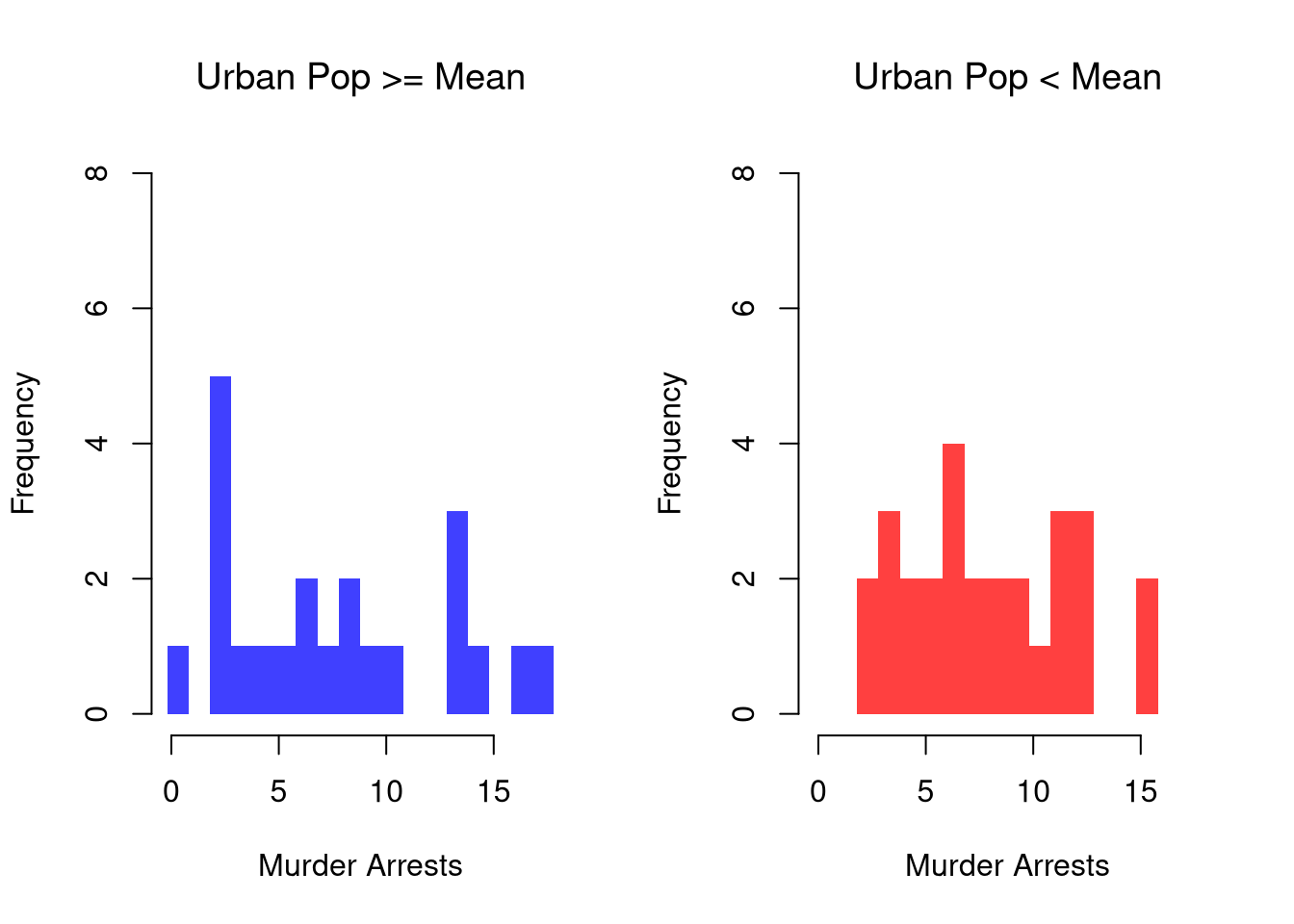
It is sometimes it is preferable to show the ECDF instead. And you can glue various combinations together to convey more information all at once
par(mfrow=c(1,2))
# Full Sample Density
hist(USArrests[,'Murder'],
    main='Density Function Estimate', font.main=1,
    xlab='Murder Arrests',
    breaks=xbks, freq=F, border=NA)

# Split Sample Distribution Comparison
F_lowpop <- ecdf(murder_lowpop)
plot(F_lowpop, col=cols[1],
    pch=16, xlab='Murder Arrests',
    main='Distribution Function Estimates',
    font.main=1, bty='n')
F_highpop <- ecdf(murder_highpop)
plot(F_highpop, add=T, col=cols[2], pch=16)

legend('bottomright', col=cols,
    pch=16, bty='n', inset=c(0,.1),
    title='% Urban Pop.',
    legend=c('Low (<= Mean)','High (>= Mean)'))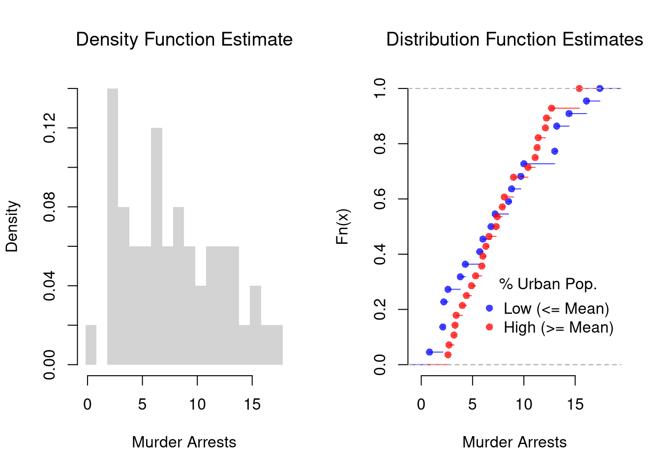
# Simple Interactive Scatter Plot
# plot(Assault~UrbanPop, USArrests, col=grey(0,.5), pch=16,
#    cex=USArrests[,'Murder']/diff(range(USArrests[,'Murder']))*2,
#    main='US Murder arrests (per 100,000)')
You can also split data into grouped boxplots in the same way
layout( t(c(1,2,2)))
boxplot(USArrests[,'Murder'], main='',
    xlab='All Data', ylab='Murder Arrests')

# K Groups with even spacing
K <- 3
USArrests[,'UrbanPop_Kcut'] <- cut(USArrests[,'UrbanPop'],K)
Kcols <- hcl.colors(K,alpha=.5)
boxplot(Murder~UrbanPop_Kcut, USArrests,
    main='', col=Kcols,
    xlab='Urban Population', ylab='')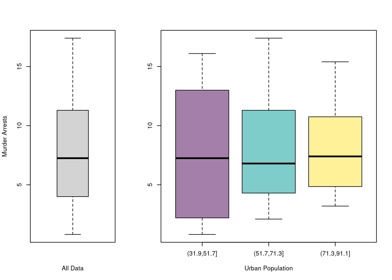
# 4 Groups with equal numbers of observations
#Qcuts <- c(
#    '0%'=min(USArrests[,'UrbanPop'])-10*.Machine[['double.eps']],
#    quantile(USArrests[,'UrbanPop'], probs=c(.25,.5,.75,1)))
#USArrests[,'UrbanPop']_cut <- cut(USArrests[,'UrbanPop'], Qcuts)
#boxplot(Murder~UrbanPop_cut, USArrests, col=hcl.colors(4,alpha=.5))There are several ways to statistically describe the relationship between two variables. The major differences surround whether the data are cardinal or an ordered/unordered factor.
Pearson (Linear) Correlation. Suppose \(X\) and \(Y\) are both cardinal data. As such, you can compute the most famous measure of association, the covariance: \[ C_{XY} = \sum_{i} [X_i - \overline{X}] [Y_i - \overline{Y}] / N \]
#plot(xy, pch=16, col=grey(0,.25))
cov(xy)
##             Murder   UrbanPop
## Murder   18.970465   4.386204
## UrbanPop  4.386204 209.518776
Note that \(C_{XX}=V_{X}\). For ease of interpretation and comparison, we rescale this statistic to always lay between \(-1\) and \(1\) \[ r_{XY} = \frac{ C_{XY} }{ \sqrt{V_X} \sqrt{V_Y}} \]
cor(xy)[2]
## [1] 0.06957262
Falk Codeviance. The Codeviance is a robust alternative to Covariance. Instead of relying on means (which can be sensitive to outliers), it uses medians (\(\tilde{X}\)) to capture the central tendency.1 We can also scale the Codeviance by the median absolute deviation to compute the median correlation. \[\begin{eqnarray} \text{CoDev}(X,Y) = \text{Med}\left\{ |X_i - \tilde{X}| |Y_i - \tilde{Y}| \right\} \\ \tilde{r}_{XY} = \frac{ \text{CoDev}(X,Y) }{ \text{MAD}(X) \text{MAD}(Y) }. \end{eqnarray}\]
cor_m <- function(xy) {
  # Compute medians for each column
  med <- apply(xy, 2, median)
  # Subtract the medians from each column
  xm <- sweep(xy, 2, med, "-")
  # Compute CoDev
  CoDev <- median(xm[, 1] * xm[, 2])
  # Compute the medians of absolute deviation
  MadProd <- prod( apply(abs(xm), 2, median) )
  # Return the robust correlation measure
  return( CoDev / MadProd)
}
cor_m(xy)
## [1] 0.005707763Suppose \(X\) and \(Y\) are both ordered variables. Kendall’s Tau measures the strength and direction of association by counting the number of concordant pairs (where the ranks agree) versus discordant pairs (where the ranks disagree). A value of \(\tau = 1\) implies perfect agreement in rankings, \(\tau = -1\) indicates perfect disagreement, and \(\tau = 0\) suggests no association in the ordering. \[ \tau = \frac{2}{n(n-1)} \sum_{i} \sum_{j > i} \text{sgn} \Bigl( (X_i - X_j)(Y_i - Y_j) \Bigr), \] where the sign function is: \[ \text{sgn}(z) = \begin{cases} +1 & \text{if } z > 0\\ 0 & \text{if } z = 0 \\ -1 & \text{if} z < 0 \end{cases}. \]
xy <- USArrests[,c('Murder','UrbanPop')]
xy[,1] <- rank(xy[,1] )
xy[,2] <- rank(xy[,2] )
# plot(xy, pch=16, col=grey(0,.25))
tau <- cor(xy[, 1], xy[, 2], method = "kendall")
round(tau, 3)
## [1] 0.074Suppose \(X\) and \(Y\) are both categorical variables; the value of \(X\) is one of \(1...r\) categories and the value of \(Y\) is one of \(1...k\) categories. Cramer’s V quantifies the strength of association by adjusting a “chi-squared” statistic to provide a measure that ranges from \(0\) to \(1\); \(0\) indicates no association while a value closer to \(1\) signifies a strong association.
First, consider a contingency table for \(X\) and \(Y\) with \(r\) rows and \(k\) columns. The chi-square statistic is then defined as:
\[ \chi^2 = \sum_{i=1}^{r} \sum_{j=1}^{k} \frac{(O_{ij} - E_{ij})^2}{E_{ij}}. \]
where
Second, normalize the chi-square statistic with the sample size and the degrees of freedom to compute Cramer’s V.
\[ V = \sqrt{\frac{\chi^2 / n}{\min(k - 1, \, r - 1)}}, \]
where:
xy <- USArrests[,c('Murder','UrbanPop')]
xy[,1] <- cut(xy[,1],3)
xy[,2] <- cut(xy[,2],4)
table(xy)
##               UrbanPop
## Murder         (31.9,46.8] (46.8,61.5] (61.5,76.2] (76.2,91.1]
##   (0.783,6.33]           4           5           8           5
##   (6.33,11.9]            0           4           7           6
##   (11.9,17.4]            2           4           2           3

cor_v <- function(xy){
    # Create a contingency table from the categorical variables
    tbl <- table(xy)
    # Compute the chi-square statistic (without Yates' continuity correction)
    chi2 <- chisq.test(tbl, correct=FALSE)[['statistic']]
    # Total sample size
    n <- sum(tbl)
    # Compute the minimum degrees of freedom (min(rows-1, columns-1))
    df_min <- min(nrow(tbl) - 1, ncol(tbl) - 1)
    # Calculate Cramer's V
    V <- sqrt((chi2 / n) / df_min)
    return(V)
}
cor_v(xy)
## X-squared
## 0.2307071

# DescTools::CramerV( table(xy) )For mixed data, where \(Y_{i}\) is a cardinal variable and \(X_{i}\) is an unordered factor variable, we analyze associations via group comparisons. You have already seen via two-sample difference, which corresponds to an \(X_{i}\) with two categories.
The joint distribution is defined as \[\begin{eqnarray} Prob(X_{i} = x, Y_{i} = y) \end{eqnarray}\] Variables are statistically independent if \(Prob(X_{i} = x, Y_{i} = y)= Prob(X_{i} = x) Prob(Y_{i} = y)\) for all \(x, y\). Independance is sometimes assumed for mathematical simplicity, not because it generally fits data well.2
The conditional distributions are defined as \[\begin{eqnarray} Prob(X_{i} = x | Y_{i} = y) = \frac{ Prob(X_{i} = x, Y_{i} = y)}{ Prob( Y_{i} = y )}\\ Prob(Y_{i} = y | X_{i} = x) = \frac{ Prob(X_{i} = x, Y_{i} = y)}{ Prob( X_{i} = x )} \end{eqnarray}\] The marginal distributions are then defined as \[\begin{eqnarray} Prob(X_{i} = x) = \sum_{y} Prob(X_{i} = x | Y_{i} = y) Prob( Y_{i} = y ) \\ Prob(Y_{i} = y) = \sum_{x} Prob(Y_{i} = y | X_{i} = x) Prob( X_{i} = x ), \end{eqnarray}\] which is also known as the law of total probability.
For one example, Consider flipping two coins. Denoted each coin as \(k \in \{1, 2\}\), and mark whether “heads” is face up; \(X_{ki}=1\) if Heads and \(=0\) if Tails. Suppose both coins are “fair”: \(Prob(X_{i}=1)= 1/2\) and \(Prob(Y_{i}=1|X_{i})=1/2\), then the four potential outcomes have equal probabilities. The joint distribution is \[\begin{eqnarray} Prob(X_{i} = x, Y_{i} = y) &=& Prob(X_{i} = x) Prob(Y_{i} = y)\\ Prob(X_{i} = 0, Y_{i} = 0) &=& 1/2 \times 1/2 = 1/4 \\ Prob(X_{i} = 0, Y_{i} = 1) &=& 1/4 \\ Prob(X_{i} = 1, Y_{i} = 0) &=& 1/4 \\ Prob(X_{i} = 1, Y_{i} = 1) &=& 1/4 . \end{eqnarray}\] The marginal distribution of the second coin is \[\begin{eqnarray} Prob(Y_{i} = 0) &=& Prob(Y_{i} = 0 | X_{i} = 0) Prob(X_{i}=0) + Prob(Y_{i} = 0 | X_{i} = 1) Prob(X_{i}=1)\\ &=& 1/2 \times 1/2 + 1/2 \times 1/2 = 1/2\\ Prob(Y_{i} = 1) &=& Prob(Y_{i} = 1 | X_{i} = 0) Prob(X_{i}=0) + Prob(Y_{i} = 1 | X_{i} = 1) Prob(X_{i}=1)\\ &=& 1/2 \times 1/2 + 1/2 \times 1/2 = 1/2 \end{eqnarray}\]
# Create a 2x2 matrix for the joint distribution.
# Rows correspond to X1 (coin 1), and columns correspond to X2 (coin 2).
P_fair <- matrix(1/4, nrow = 2, ncol = 2)
rownames(P_fair) <- c("X1=0", "X1=1")
colnames(P_fair) <- c("X2=0", "X2=1")
P_fair
##      X2=0 X2=1
## X1=0 0.25 0.25
## X1=1 0.25 0.25

# Compute the marginal distributions.
# Marginal for X1: sum across columns.
P_X1 <- rowSums(P_fair)
P_X1
## X1=0 X1=1
##  0.5  0.5
# Marginal for X2: sum across rows.
P_X2 <- colSums(P_fair)
P_X2
## X2=0 X2=1
##  0.5  0.5

# Compute the conditional probabilities Prob(X2 | X1).
cond_X2_given_X1 <- matrix(0, nrow = 2, ncol = 2)
for (j in 1:2) {
  cond_X2_given_X1[, j] <- P_fair[, j] / P_X1[j]
}
rownames(cond_X2_given_X1) <- c("X2=0", "X2=1")
colnames(cond_X2_given_X1) <- c("given X1=0", "given X1=1")
cond_X2_given_X1
##      given X1=0 given X1=1
## X2=0        0.5        0.5
## X2=1 0.5 0.5Consider a second example, where the second coin is “Completely Unfair”, so that it is always the same as the first. The outcomes generated with a Completely Unfair coin are the same as if we only flipped one coin. \[\begin{eqnarray} Prob(X_{i} = x, Y_{i} = y) &=& Prob(X_{i} = x) \mathbf{1}( x=y )\\ Prob(X_{i} = 0, Y_{i} = 0) &=& 1/2 \\ Prob(X_{i} = 0, Y_{i} = 1) &=& 0 \\ Prob(X_{i} = 1, Y_{i} = 0) &=& 0 \\ Prob(X_{i} = 1, Y_{i} = 1) &=& 1/2 . \end{eqnarray}\] Note that \(\mathbf{1}(X_{i}=1)\) means \(X_{i}= 1\) and \(0\) if \(X_{i}\neq0\). The marginal distribution of the second coin is \[\begin{eqnarray} Prob(Y_{i} = 0) &=& Prob(Y_{i} = 0 | X_{i} = 0) Prob(X_{i}=0) + Prob(Y_{i} = 0 | X_{i} = 1) Prob(X_{i} = 1)\\ &=& 1/2 \times 1 + 0 \times 1/2 = 1/2 .\\ Prob(Y_{i} = 1) &=& Prob(Y_{i} = 1 | X_{i} =0) Prob( X_{i} = 0) + Prob(Y_{i} = 1 | X_{i} = 1) Prob( X_{i} = 1)\\ &=& 0\times 1/2 + 1 \times 1/2 = 1/2 . \end{eqnarray}\] which is the same as in the first example! Different joint distributions can have the same marginal distributions.
# Create the joint distribution matrix for the unfair coin case.
P_unfair <- matrix(c(0.5, 0, 0, 0.5), nrow = 2, ncol = 2, byrow = TRUE)
rownames(P_unfair) <- c("X1=0", "X1=1")
colnames(P_unfair) <- c("X2=0", "X2=1")
P_unfair
##      X2=0 X2=1
## X1=0  0.5  0.0
## X1=1  0.0  0.5

# Compute the marginal distribution for X2 in the unfair case.
P_X2_unfair <- colSums(P_unfair)
P_X1_unfair <- rowSums(P_unfair)

# Compute the conditional probabilities Prob(X1 | X2) for the unfair coin.
cond_X2_given_X1_unfair <- matrix(NA, nrow = 2, ncol = 2)
for (j in 1:2) {
  if (P_X1_unfair[j] > 0) {
    cond_X2_given_X1_unfair[, j] <- P_unfair[, j] / P_X1_unfair[j]
  }
}
rownames(cond_X2_given_X1_unfair) <- c("X2=0", "X2=1")
colnames(cond_X2_given_X1_unfair) <- c("given X1=0", "given X1=1")
cond_X2_given_X1_unfair
##      given X1=0 given X1=1
## X2=0          1          0
## X2=1 0 1The joint distribution is defined as \[\begin{eqnarray} F(x, y) &=& Prob(X_{i} \leq x, Y_{i} \leq y) \end{eqnarray}\] The marginal distributions are then defined as \[\begin{eqnarray} F_{X}(x) &=& F(x, \infty)\\ F_{Y}(y) &=& F(\infty, y). \end{eqnarray}\] which is also known as the law of total probability. Variables are statistically independent if \(F(x, y) = F_{X}(x)F_{Y}(y)\) for all \(x, y\).
For example, suppose \((X_{i},Y_{i})\) is bivariate normal with means \((\mu_{X}, \mu_{Y})\), variances \((\sigma_{X}, \sigma_{Y})\) and covariance \(\rho\).
# Simulate Bivariate Data
N <- 10000
Mu <- c(2,2) ## Means

Sigma1 <- matrix(c(2,-.8,-.8,1),2,2) ## CoVariance Matrix
MVdat1 <- mvtnorm::rmvnorm(N, Mu, Sigma1)

Sigma2 <- matrix(c(2,.4,.4,1),2,2) ## CoVariance Matrix
MVdat2 <- mvtnorm::rmvnorm(N, Mu, Sigma2)

par(mfrow=c(1,2))
## Different diagonals
plot(MVdat2, col=rgb(1,0,0,0.02), pch=16,
    main='Joint', font.main=1,
    ylim=c(-4,8), xlim=c(-4,8), xlab='X1', ylab='X2')
points(MVdat1,col=rgb(0,0,1,0.02),pch=16)
## Same marginal distributions
xbks <- seq(-4,8,by=.2)
hist(MVdat2[,2], col=rgb(1,0,0,0.5),
    breaks=xbks, border=NA, xlab='X2',
    main='Marginal', font.main=1)
hist(MVdat1[,2], col=rgb(0,0,1,0.5),
    add=T, breaks=xbks, border=NA)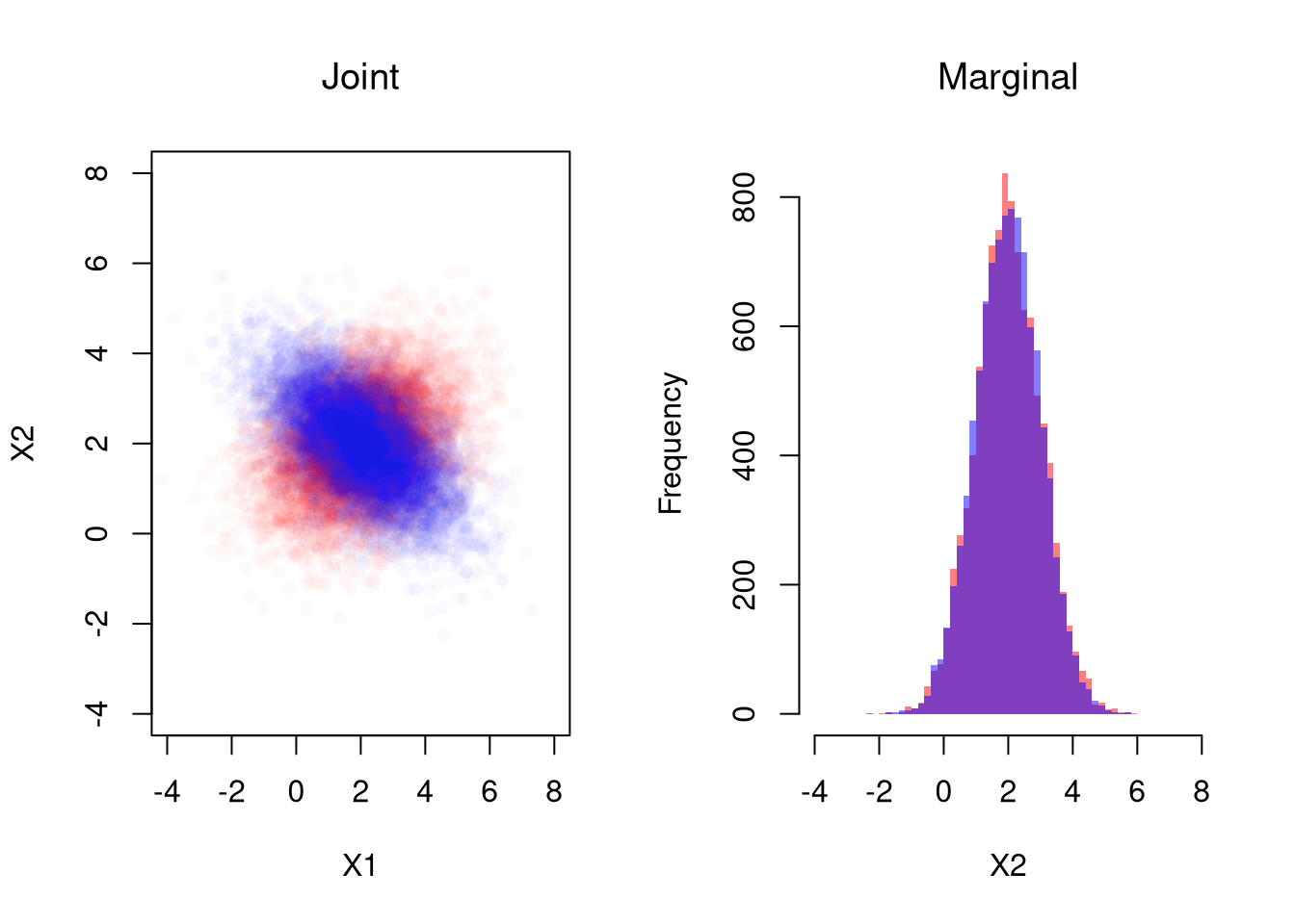
# See that independent data are a special case
n <- 2e4
## 2 Indepenant RV
XYiid <- cbind( rnorm(n),  rnorm(n))
## As a single Joint Draw
XYjoint <- mvtnorm::rmvnorm(n, c(0,0))
## Plot
par(mfrow=c(1,2))
plot(XYiid, xlab=
    col=grey(0,.05), pch=16, xlim=c(-5,5), ylim=c(-5,5))
plot(XYjoint,
    col=grey(0,.05), pch=16, xlim=c(-5,5), ylim=c(-5,5))

# Compare densities
#d1 <- dnorm(XYiid[,1],0)*dnorm(XYiid[,2],0)
#d2 <- mvtnorm::dmvnorm(XYiid, c(0,0))
#head(cbind(d1,d2))
The multivariate normal is a workhorse for analytical work on multivariate random variables, but there are many more. See e.g., https://cran.r-project.org/web/packages/NonNorMvtDist/NonNorMvtDist.pdf
Note Simpson’s Paradox:
Also note Bayes’ Theorem: \[\begin{eqnarray} Prob(X_{i} = x | Y_{i} = y) Prob( Y_{i} = y) &=& Prob(X_{i} = x, Y_{i} = y) = Prob(Y_{i} = y | X_{i} = x) Prob(X_{i} = x).\\ Prob(X_{i} = x | Y_{i} = y) &=& \frac{ Prob(Y_{i} = y | X_{i} = x) Prob(X_{i}=x) }{ Prob( Y_{i} = y) }. \end{eqnarray}\]
# Verify Bayes' theorem for the unfair coin case:
# Compute Prob(X1=1 | X2=1) using the formula:
#   Prob(X1=1 | X2=1) = [Prob(X2=1 | X1=1) * Prob(X1=1)] / Prob(X2=1)

P_X1_1 <- 0.5
P_X2_1_given_X1_1 <- 1  # Since coin 2 copies coin 1.
P_X2_1 <- P_X2_unfair["X2=1"]

bayes_result <- (P_X2_1_given_X1_1 * P_X1_1) / P_X2_1
bayes_result
## X2=1
## 1For plotting histograms and marginal distributions, see
Many introductory econometrics textbooks have a good appendix on probability and statistics. There are many useful statistical texts online too
See the Further reading about Probability Theory in the Statistics chapter.
Other Statistics