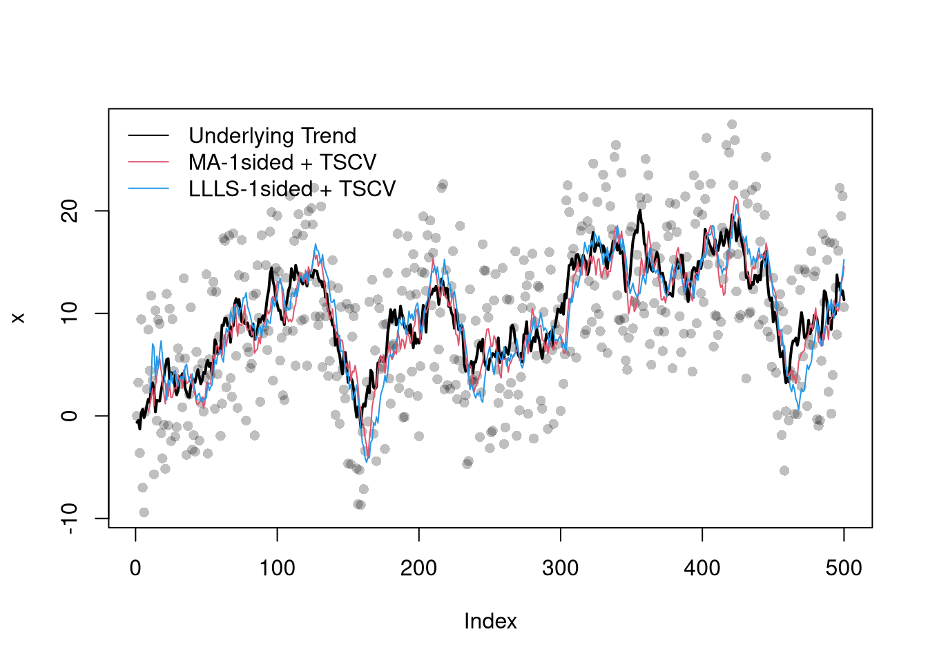
17 Misc. Topics

17.1 Nonparametric Tests

Distributional Comparisons.

We can also examine whether there are any differences between the entire distributions

Code

# Sample Wage Data
library(wooldridge)
x1 <- sort( wage1[wage1$educ == 15,  'wage'])  
x2 <- sort( wage1[wage1$educ == 16,  'wage'] )
x <- sort(c(x1, x2))

# Compute Quantiles
quants <- seq(0,1,length.out=101)
Q1 <- quantile(x1, probs=quants)
Q2 <- quantile(x2, probs=quants)

# Compare Distributions via Quantiles
rx <- range(c(x1, x2))
par(mfrow=c(1,2))
plot(rx, c(0,1), type='n', font.main=1,
    main='Distributional Comparison',
    xlab=expression(Q[s]),
    ylab=expression(F[s]))
lines(Q1, quants, col=2)
lines(Q2, quants, col=4)
legend('bottomright', col=c(2,4), lty=1,
legend=c('F1', 'F2'))

# Compare Quantiles
plot(Q1, Q2, xlim=rx, ylim=rx,
    main='Quantile-Quantile Plot', font.main=1,
pch=16, col=grey(0,.25))
abline(a=0,b=1,lty=2)

The starting point for hypothesis testing is the Kolmogorov-Smirnov Statistic: the maximum absolute difference between two CDF’s over all sample data \(x \in \{X_1\} \cup \{X_2\}\). \[\begin{eqnarray} KS &=& \max_{x} |F_{1}(x)- F_{2}(x)|^{p}, \end{eqnarray}\] where \(p\) is an integer (typically 1). An intuitive alternative is the Cramer-von Mises Statistic: the sum of absolute differences (raised to an integer, typically 2) between two CDF’s. \[\begin{eqnarray} CVM=\sum_{x} |F_{1}(x)- F_{2}(x)|^{p}. \end{eqnarray}\]

Code

# Distributions
F1 <- ecdf(x1)(x)
F2 <- ecdf(x2)(x)

library(twosamples)

# Kolmogorov-Smirnov
KSq <- which.max(abs(F2 - F1))
KSqv <- round(twosamples::ks_stat(x1, x2),2)

# Cramer-von Mises Statistic (p=2)
CVMqv <- round(twosamples::cvm_stat(x1, x2, power=2), 2) 

# Visualize Differences
plot(range(x), c(0,1), type="n", xlab='x', ylab='ECDF')
lines(x, F1, col=2, lwd=2)
lines(x, F2, col=4, lwd=2)
# CVM
segments(x, F1, x, F2, lwd=.5, col=grey(0,.2))
# KS
segments(x[KSq], F1[KSq], x[KSq], F2[KSq], lwd=1.5, col=grey(0,.75), lty=2)

Just as before, you use bootstrapping for hypothesis testing.

Code

twosamples::cvm_test(x1, x2)
## Test Stat   P-Value 
##  2.084253  0.084500

Comparing Multiple Groups.

For multiple groups, we can tests the equality of all distributions (whether at least one group is different). The Kruskal-Wallis test examines \(H_0:\; F_1 = F_2 = \dots = F_G\) versus \(H_A:\; \text{at least one } F_g \text{ differs}\), where \(F_g\) is the continuous distribution of group \(g=1,...G\). This test does not tell us which group is different.

To conduct the test, first denote individuals \(i=1,...n\) with overall ranks \(r_1,....r_{n}\). Each individual belongs to group \(g=1,...G\), and each group \(g\) has \(n_{g}\) individuals with average rank \(\overline{r}_{g} = \sum_{i} r_{i} /n_{g}\). The Kruskal Wallis statistic is \[\begin{eqnarray} KW &=& (N-1) \frac{\sum_{g=1}^{G} n_{g}( \overline{r}_{g} - \overline{r} )^2 }{\sum_{i=1}^{N} ( r_{i} - \overline{r} )^2}, \end{eqnarray}\] where \(\overline{r} = \frac{N+1}{2}\) is the grand mean rank.

In the special case with only two groups, \(G=2\), the Kruskal Wallis test reduces to the Mann–Whitney U-test (also known as the ). In this case, we can write the hypotheses in terms of individual outcomes in each group, \(Y_i\) in one group \(Y_j\) in the other; \(H_0: P(Y_i > Y_j)=P(Y_i > Y_i)\) versus \(H_A: P(Y_i > Y_j) \neq P(Y_i > Y_j)\). The corresponding test statistic is \[\begin{eqnarray} U &=& \min(U_1,U_2) \\ U_g &=& \sum_{i\in g}\sum_{j\in -g} \Bigl[\mathbf 1(Y_i > Y_j) + \tfrac12\mathbf 1(Y_i = Y_j)\Bigr]. \end{eqnarray}\]

Code

library(AER)
data(CASchools)
CASchools$stratio <- CASchools$students/CASchools$teachers

# Do student/teacher ratio differ for at least 1 county?
# Single test of multiple distributions
kruskal.test(CASchools$stratio, CASchools$county)
## 
##  Kruskal-Wallis rank sum test
## 
## data:  CASchools$stratio and CASchools$county
## Kruskal-Wallis chi-squared = 161.18, df = 44, p-value = 2.831e-15

# Multiple pairwise tests
# pairwise.wilcox.test(CASchools$stratio, CASchools$county)

17.2 Predictions

Describe vs. Explain vs. Predict.

Prediction Intervals.

In addition to confidence intervals, we can also compute a prediction interval which estimate the variability of new data rather than a statistic

In this example, we consider a single variable and compute the frequency each value was covered.

Code

x <- runif(1000)
# Middle 90% of values
xq0 <- quantile(x, probs=c(.05,.95))

bks <- seq(0,1,by=.01)
hist(x, breaks=bks, border=NA,
    main='Prediction Interval', font.main=1)
abline(v=xq0)

Code


paste0('we are 90% confident that the a future data point will be between ', 
    round(xq0[1],2), ' and ', round(xq0[2],2) )
## [1] "we are 90% confident that the a future data point will be between 0.06 and 0.96"

In this example, we consider a range for \(y_{i}(x)\) rather than for \(m(x)\). These intervals also take into account the residuals — the variability of individuals around the mean.

Code

# Bivariate Data from USArrests
xy <- USArrests[,c('Murder','UrbanPop')]
colnames(xy) <- c('y','x')
xy0 <- xy[order(xy$x),]

For a nice overview of different types of intervals, see https://www.jstor.org/stable/2685212. For an in-depth view, see “Statistical Intervals: A Guide for Practitioners and Researchers” or “Statistical Tolerance Regions: Theory, Applications, and Computation”. See https://robjhyndman.com/hyndsight/intervals/ for constructing intervals for future observations in a time-series context. See Davison and Hinkley, chapters 5 and 6 (also Efron and Tibshirani, or Wehrens et al.)

Code

# From "Basic Regression"
xy0 <- xy[order(xy$x),]
X0 <- unique(xy0$x)
reg_lo <- loess(y~x, data=xy0, span=.8)
preds_lo <- predict(reg_lo, newdata=data.frame(x=X0))


# Jackknife CI
jack_lo <- sapply(1:nrow(xy), function(i){
    xy_i <- xy[-i,]
    reg_i <- loess(y~x, dat=xy_i, span=.8)
    predict(reg_i, newdata=data.frame(x=X0))
})

boot_regs <- lapply(1:399, function(b){
    b_id <- sample( nrow(xy), replace=T)
    xy_b <- xy[b_id,]
    reg_b <- lm(y~x, dat=xy_b)
})

plot(y~x, pch=16, col=grey(0,.5),
    dat=xy0, ylim=c(0, 20))
lines(X0, preds_lo,
    col=hcl.colors(3,alpha=.75)[2],
    type='o', pch=2)

# Estimate Residuals CI at design points
res_lo <- sapply(1:nrow(xy), function(i){
    y_i <- xy[i,'y']
    preds_i <- jack_lo[,i]
    resids_i <- y_i - preds_i
})
res_cb <- apply(res_lo, 1, quantile,
    probs=c(.025,.975), na.rm=T)

# Plot
lines( X0, preds_lo +res_cb[1,],
    col=hcl.colors(3,alpha=.75)[2], lt=2)
lines( X0, preds_lo +res_cb[2,],
    col=hcl.colors(3,alpha=.75)[2], lty=2)



# Smooth estimates 
res_lo <- lapply(1:nrow(xy), function(i){
    y_i <- xy[i,'y']
    x_i <- xy[i,'x']
    preds_i <- jack_lo[,i]
    resids_i <- y_i - preds_i
    cbind(e=resids_i, x=x_i)
})
res_lo <- as.data.frame(do.call(rbind, res_lo))

res_fun <- function(x0, h, res_lo){
    # Assign equal weight to observations within h distance to x0
    # 0 weight for all other observations
    ki <- dunif(res_lo$x, x0-h, x0+h) 
    ei <- res_lo[ki!=0,'e']
    res_i <- quantile(ei, probs=c(.025,.975), na.rm=T)
}
res_lo2 <- sapply(X0, res_fun, h=15, res_lo=res_lo)

lines( X0, preds_lo + res_lo2[1,],
    col=hcl.colors(3,alpha=.75)[2], lty=1, lwd=2)
lines( X0, preds_lo + res_lo2[2,],
    col=hcl.colors(3,alpha=.75)[2], lty=1, lwd=2)

Code

# Bootstrap Prediction Interval
boot_resids <- lapply(boot_regs, function(reg_b){
    e_b <- resid(reg_b)
    x_b <- reg_b$model$x
    res_b <- cbind(e_b, x_b)
})
boot_resids <- as.data.frame(do.call(rbind, boot_resids))
# Homoskedastic
ehat <- quantile(boot_resids$e_b, probs=c(.025, .975))
x <- quantile(xy$x,probs=seq(0,1,by=.1))
boot_pi <- coef(reg)[1] + x*coef(reg)['x']
boot_pi <- cbind(boot_pi + ehat[1], boot_pi + ehat[2])

# Plot Bootstrap PI
plot(y~x, dat=xy, pch=16, main='Prediction Intervals',
    ylim=c(-5,20), font.main=1)
polygon( c(x, rev(x)), c(boot_pi[,1], rev(boot_pi[,2])),
    col=grey(0,.2), border=NA)

# Parametric PI (For Comparison)
#pi <- predict(reg, interval='prediction', newdata=data.frame(x))
#lines( x, pi[,'lwr'], lty=2)
#lines( x, pi[,'upr'], lty=2)

Crossvalidation.

Perhaps the most common approach to selecting a bandwidth is to minimize error. Leave-one-out Cross-validation minimizes the average “leave-one-out” mean square prediction errors: \[\begin{eqnarray} CV &=& \min_{\mathbf{H}} \quad \frac{1}{n} \sum_{i=1}^{n} \left[ Y_{i} - \widehat{Y_{[i]}}(\mathbf{X},\mathbf{H}) \right]^2, % \widehat{Y_{[i]}}(\mathbf{X},\mathbf{H}) &=& \sum_{j\neq i} k(\mathbf{X}_{j},\mathbf{X}_{i},\mathbf{H}) \left[ \widehat{\alpha}(\mathbf{X}_{j}) + \widehat{\beta}(\mathbf{X}_{j}) \mathbf{X}_{i} \right] \end{eqnarray}\] where \(\widehat{Y_{[i]}}(\mathbf{X},\mathbf{H})\) is the predicted value at \(\mathbf{X}_{i}\) based on a dataset that excludes \(\mathbf{X}_{i}\).

There are many types of cross-validation . For example, one extension is , which splits \(N\) datapoints into \(k=1...K\) groups, each sized \(B\), and predicts values for the left-out group. adjusts for the degrees of freedom, whereas the function in R uses by default. You can refer to extensions on a case by case basis.

Minimizing out-sample prediction error is perhaps the simplest computational approach to choose bandwidths, and it also addresses an issue that plagues observational studies in the social sciences of explanations without predictions. It is a problem if your model explains everything and predicts nothing, but minimizing prediction error is not necessarily “best”.

Code

##################                                         
# Crossvalidated bandwidth for regression
##################
y <- (CASchools$read + CASchools$math) / 2
xy_mat <- data.frame(y=y, x1=CASchools$income)
library(np)

## Grid Search
BWS <- seq(1,10,length.out=20)
BWS_CV <- sapply(BWS, function(bw){
    E_bw <- sapply(1:nrow(xy_mat), function(i){
        llls <- npreg(y~x1, data=xy_mat[-i,], 
            bws=bw, regtype="ll",
            ckertype='epanechnikov', bandwidth.compute=F)
        pred_i <- predict(llls, newdata=xy_mat[i,])
        e <-  (pred_i- xy_mat[i,'y'])
        return(e)
    })
    return( mean(E_bw^2) )
})

## Plot MSE
par(mfrow=c(1,2))
plot(BWS, BWS_CV, ylab='CV', pch=16, 
    xlab='bandwidth (h)',)
## Plot Resulting Predictions
bw <- BWS[which.min(BWS_CV)]
llls <- npreg(y~x1, data=xy_mat, 
    ckertype='epanechnikov',
    bws=bw, regtype="ll")
plot(xy_mat$x, predict(llls), pch=16, col=grey(0,.5),
    xlab='X', ylab='Predictions')
abline(a=0,b=1, lty=2)

## Built in algorithmic Optimziation
llls2 <- npreg(y~x1, data=xy_mat, ckertype='epanechnikov', regtype="ll")
points(xy_mat$x, predict(llls2), pch=2, col=rgb(1,0,0,.25))

## Add legend
add_legend <- function(...) {
  opar <- par(fig=c(0, 1, 0, 1), oma=c(0, 0, 0, 0), 
              mar=c(0, 0, 0, 0), new=TRUE)
  on.exit(par(opar))
  plot(0, 0, type='n', bty='n', xaxt='n', yaxt='n')
  legend(...)
}
add_legend('topright',
    col=c(grey(0,.5),rgb(1,0,0,.25)), 
    pch=c(16,2),
    bty='n', horiz=T,
    legend=c('Grid Search', 'NP-algorithm'))

Code

##################
# CV Application
##################

## Smoothly Estimate X & Y Density
y <- sort(xy_mat$y)
fy <- npudens(y, bandwidth.compute=TRUE)
x1 <- sort(xy_mat$x1)
fx <- npudens(x1, bandwidth.compute=TRUE)
## Smoothly Estimate How Y changes with X
llls2 <- npreg(y~x1,data=xy_mat,
    ckertype='epanechnikov',
    regtype="ll", bandwidth.compute=TRUE)


layout( matrix(c(2,0,1,3), ncol=2, byrow=TRUE),
    widths=c(4/5,1/5), heights=c(1/5,4/5))
## Joint Distribution
par(mar=c(4,4,1,1))
plot(y~x1, data=xy_mat,
    pch=16, col=grey(0,.25),
    xlab="District Income (1000$)", 
    ylab="Test Score")
lines( sort(xy_mat$x), predict(llls2)[order(xy_mat$x1)],
    pch=16, col=1)
## Marginal Distribution
par(mar=c(0,4,1,1))
plot(x1, predict(fx),
    col=grey(0,1), type='l', axes=F,
    xlab='', ylab='')
rug(x1, col=grey(0,.25))
par(mar=c(4,0,1,1))
plot(predict(fy), y,
    col=grey(0,1), type='l', axes=F,
    xlab='', ylab='')
rug(y, col=grey(0,.25), side=2)

Filtering.

In some cases, we may want to smooth time series data instead of predict into the future. We can distinguish two types of smoothing, incorporating future observations or not. When only weighting two other observations, the differences can be expressed as trying to estimate the average with different available data:

Filtering: \(\mathbb{E}[Y_{t} | X_{t-1}, X_{t-2}]\)
Smoothing: \(\mathbb{E}[Y_{t} | X_{t-1}, X_{t+1}]\)

One example of filtering is Exponential Filtering (sometimes confusingly referred to as “Exponential Smoothing”) which weights only previous observations using an exponential kernel.

Code

##################
# Time series data
##################

set.seed(1)
## Underlying Trend
x0 <- cumsum(rnorm(500,0,1))
## Observed Datapoints
x <- x0 + runif(length(x0),-10,10)
dat <- data.frame(t=seq(x), x0=x0, x=x)

## Asymmetric Kernel
#bw <- c(2/3,1/3)
#s1 <- filter(x, bw/sum(bw), sides=1)

## Symmetric Kernel
#bw <- c(1/6,2/3,1/6)
#s2 <- filter(x,  bw/sum(bw), sides=2)

There are several cross-validation procedures for filtering time series data . One is called time series cross-validation (TSCV), which is useful for temporally dependent data .

Code

## Plot Simulated Data
x <- dat$x
x0 <- dat$x0
par(fig = c(0,1,0,1), new=F)
plot(x, pch=16, col=grey(0,.25))
lines(x0, col=1, lty=1, lwd=2)

## Work with differenced data?
#n       <- length(Yt)
#plot(Yt[1:(n-1)], Yt[2:n],
#    xlab='d Y (t-1)', ylab='d Y (t)', 
#    col=grey(0,.5), pch=16)
#Yt <- diff(Yt)

## TSCV One Sided Moving Average
filter_bws <- seq(1,20,by=1)
filter_mape_bws <- sapply(filter_bws, function(h){
    bw <- c(0,rep(1/h,h)) ## Leave current one out
    s2 <- filter(x, bw, sides=1)
    pe <- s2 - x
    mape <- mean( abs(pe)^2, na.rm=T)
})
filter_mape_star <- filter_mape_bws[which.min(filter_mape_bws)]
filter_h_star <- filter_bws[which.min(filter_mape_bws)]
filter_tscv <- filter(x,  c(rep(1/filter_h_star,filter_h_star)), sides=1)
# Plot Optimization Results
#par(fig = c(0.07, 0.35, 0.07, 0.35), new=T) 
#plot(filter_bws, filter_mape_bws, type='o', ylab='mape', pch=16)
#points(filter_h_star, filter_mape_star, pch=19, col=2, cex=1.5)

## TSCV for LLLS
library(np)
llls_bws <- seq(8,28,by=1)
llls_burnin <- 10
llls_mape_bws <- sapply(llls_bws, function(h){ # cat(h,'\n')
    pe <- sapply(llls_burnin:nrow(dat), function(t_end){
        dat_t <- dat[dat$t<t_end, ]
        reg <- npreg(x~t, data=dat_t, bws=h,
            ckertype='epanechnikov',
            bandwidth.compute=F, regtype='ll')
        edat <- dat[dat$t==t_end,]
        pred <- predict(reg, newdata=edat)
        pe <- edat$x - pred
        return(pe)    
    })
    mape <- mean( abs(pe)^2, na.rm=T)
})
llls_mape_star <- llls_mape_bws[which.min(llls_mape_bws)]
llls_h_star <- llls_bws[which.min(llls_mape_bws)]
#llls_tscv <- predict( npreg(x~t, data=dat, bws=llls_h_star,
#    bandwidth.compute=F, regtype='ll', ckertype='epanechnikov'))
llls_tscv <- sapply(llls_burnin:nrow(dat), function(t_end, h=llls_h_star){
    dat_t <- dat[dat$t<t_end, ]
    reg <- npreg(x~t, data=dat_t, bws=h,
        ckertype='epanechnikov',
        bandwidth.compute=F, regtype='ll')
    edat <- dat[dat$t==t_end,]
    pred <- predict(reg, newdata=edat)
    return(pred)    
})

## Compare Fits Qualitatively
lines(filter_tscv, col=2, lty=1, lwd=1)
lines(llls_burnin:nrow(dat), llls_tscv, col=4, lty=1, lwd=1)
legend('topleft', lty=1, col=c(1,2,4), bty='n',
    c('Underlying Trend', 'MA-1sided + TSCV', 'LLLS-1sided + TSCV'))

Code


## Compare Fits Quantitatively
cbind(
    bandwidth=c(LLLS=llls_h_star, MA=filter_h_star),
    mape=round(c(LLLS=llls_mape_star, MA=filter_mape_star),2) )
##      bandwidth  mape
## LLLS        18 43.39
## MA           9 42.28

## See also https://cran.r-project.org/web/packages/smoots/smoots.pdf
#https://otexts.com/fpp3/tscv.html
#https://robjhyndman.com/hyndsight/tscvexample/

17 Misc. Topics

17.1 Nonparametric Tests

Distributional Comparisons.

Comparing Multiple Groups.

17.2 Predictions

Describe vs. Explain vs. Predict.

Prediction Intervals.

Crossvalidation.

Filtering.

17.3 Decision Theory

Statistical Power

Quality Control

Optimal Experiment Designs