7  Confidence Intervals

---

The sampling distribution describes how the statistic varies across samples. The confidence interval is a way to turn knowledge about that sampling distribution into a statement about the unknown parameter. We use our sample data to construct an interval that says “we are \(Z\%\) confident that the mean is in this interval”. Just as with standard errors, we can make confidence intervals using theory-driven or data-driven approaches. We will focus on data-driven approaches first, then theory-driven approaches, then theoretical properties of confidence intervals.

7.1 Resampling Intervals

Often, we have only one sample. In practice, we can use resampling procedures to estimate a confidence interval. E.g., we repeatedly resample data and construct a bootstrap or jackknife sampling distribution. Then we compute the confidence intervals using the upper and lower quantiles of the sampling distribution. The quantiles associated with \(Z\%\) are called the critical values

• The \(5^{th}\) and \(95^{th}\) percentiles are the critical values for the \(90\%\) confidence interval.
• The \(2.5^{th}\) and \(97.5^{th}\) percentiles are the critical values for the \(95\%\) confidence interval.
• The \(0.5^{th}\) and \(99.5^{th}\) percentiles are the critical values for the \(99\%\) confidence interval.

sample_dat <- USArrests[, 'Murder']
sample_mean <- mean(sample_dat)
sample_mean
## [1] 7.788

# Bootstrap Distribution
set.seed(1) # to be replicable
bootstrap_means <- rep(NA, 9999)
for(b in seq_along(bootstrap_means)){
    dat_id <- seq_along(sample_dat)
    boot_id <- sample(dat_id , replace=T)
    dat_b  <- sample_dat[boot_id] # c.f. jackknife
    mean_b <- mean(dat_b)
    bootstrap_means[b] <-mean_b
}

# 95% CI
boot_ci <- quantile(bootstrap_means, probs=c(.025, .975), na.rm=T)
boot_ci
##   2.5%  97.5% 
## 6.6039 8.9420

# Visualize
hist(bootstrap_means, freq=F,
    main=NA,
    border=NA, breaks=50)
title('Bootstrap CI', font.main=1)
abline(v=boot_ci)

NoteMust Know

Compute a \(90%\) CI and a \(99%\) CI. Interpret each one separately, then compare the two.

This approach can be easily extended to other statistics. For example, a \(Z\%\) confidence interval for the median is an interval where \(Z\%\) of those generated will contain the population median.

TipTest Yourself

The following code creates a bootstrap CI for the median. Edit it to create a jackknife CI instead. Then edit it to create a bootstrap CI for the upper quartile.

sample_dat <- USArrests[, 'Murder']
sample_stat <- quantile(sample_dat, probs=0.5) #median
sample_stat
##  50% 
## 7.25

# Bootstrap Distribution
set.seed(1) # to be replicable
bootstrap_stats <- rep(NA, 9999)
for(b in seq_along(bootstrap_stats)){
    dat_id <- seq_along(sample_dat)
    boot_id <- sample(dat_id, replace=T)
    dat_b  <- sample_dat[boot_id] # c.f. jackknife
    stat_b <- quantile(dat_b, probs=0.5)
    bootstrap_stats[b] <-stat_b
}

# 95% CI
boot_ci <- quantile(bootstrap_stats, probs=c(.025, .975), na.rm=T)
boot_ci
##  2.5% 97.5% 
##  5.85  9.00

# Visualize
hist(bootstrap_stats, freq=F,
    main=NA,
    border=NA, breaks=50)
title('Bootstrap CI', font.main=1)
abline(v=boot_ci)

7.2 Normal Approximation

Given the sampling distribution is approximately Normal, the usual confidence intervals are symmetric. For the sample mean \(M\), we can then construct the interval \([M - E, M + E]\), where \(E\) is a margin of error on either side of \(M\). The margin of error for the Normal distribution is theoretically known, and can be calculated based on standard errors and the critical values. Given a standard error \(SE(M)\) and quantiles \(q(\alpha/2)\), we know from theory that \(E=q(\alpha/2)\cdot SE(M)\). The critical values define the Normal confidence interval associated with \(1-\alpha\) coverage, referred to above as \(Z\%\). \[\begin{eqnarray} M \pm q(\alpha/2) \cdot SE(M) \end{eqnarray}\]

A coverage level of \(1-\alpha\) means that if the same sampling procedure were repeated \(100\) times from the same population, approximately \(1-\alpha\) percent of the intervals are expected to contain the true population mean. ¹ We can also compute from theory that \(\pm 1.96~ SE(M)\) corresponds to the critical values of the Normal distribution, where \(SE(M)\) is estimated using the bootstrap distribution or theory (classical SEs: \(\hat{S}/\sqrt{n}\)). The \(95\%\) interval is the most common, and has quantile value \(q=1.96\). The \(90\%\) interval has quantile value \(q=1.65\). The values for \(M\) and \(SE(M)\) are estimated from data.

NoteMust Know

For example, suppose we sample \(n=36\) monthly electricity bills (in dollars) and find \(\hat{M}=142\) and \(\hat{S}=30\). The classical standard error is \(SE(M) \approx \hat{S}/\sqrt{n} = 30/\sqrt{36} = 5\). From theory, we also know that \(95\%\) confidence interval has upper and lower critical value of \[\begin{eqnarray} F^{-1}_{Normal}\left(0.975, SE(M) \right) &=& +1.96 \cdot SE(M) \\ F^{-1}_{Normal}\left(0.025, SE(M) \right) &=& -1.96 \cdot SE(M) \end{eqnarray}\] Together, we can calculate \[\begin{eqnarray} E &=& q(\alpha/2) \cdot SE(M) = 1.96 \cdot 5 = 9.8\\ [\hat{M} - E, \hat{M} + E] &=& [142 - 9.8, 142 + 9.8] = [132.2,~ 151.8]. \end{eqnarray}\] We are \(95\%\) confident that the population mean electricity bill is between \(\$132.20\) and \(\$151.80\).

M_hat <- 142
S_hat <- 30
n <- 36
SE <- S_hat / sqrt(n)
SE
## [1] 5

# 95% CI Manual Calculation
M_hat + c(-1.96, 1.96) * SE
## [1] 132.2 151.8

## 95% CI Intuition
qnorm( c(0.025, 0.975), M_hat, SE)
## [1] 132.2002 151.7998

The main advantages of the Normal approximation is that

• can be computed formulaically as above
• works well for estimating extreme probabilities, where resampling methods tend to be worse.

The main disadvantage is that

• the sampling distribution might be far from normal.

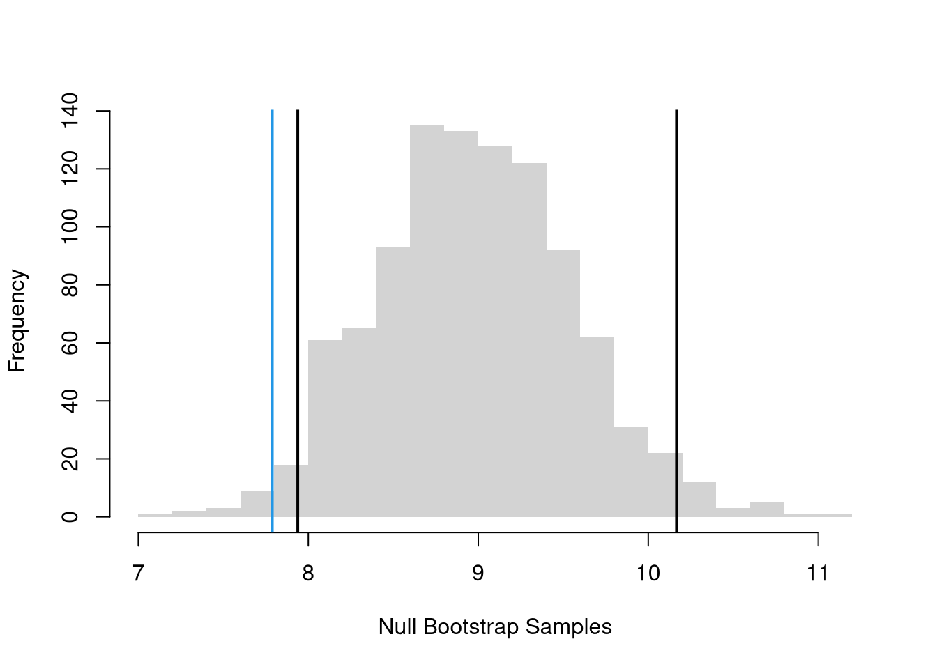
In the example below, they are all quite similar, but that does not always need to be the case.

# Bootstrap Distribution with Percentile CI
hist(bootstrap_means, breaks=25,
    main=NA, border=NA,
    freq=F, ylim=c(0, 0.7),
    xlab=expression(hat(b)[b]))
title('Percentile vs Normal 95% CIs', font.main=1)
boot_ci_percentile <- quantile(bootstrap_means, probs=c(.025, .975))
abline(v=boot_ci_percentile, lty=1)

# Normal Approximation with IID Theory SEs
classic_se <- sd(sample_dat)/sqrt(length(sample_dat))
x <- seq(5, 10, by=0.01)
fx2 <- dnorm(x, sample_mean, classic_se)
lines(x, fx2, col=rgb(1, 0, 0, .8), lty=1)
ci_normal <- qnorm(c(.025, .975), sample_mean, classic_se)
#ci_normal <- sample_mean+c(-1.96, +1.96)*classic_se
abline(v=ci_normal, col=rgb(1, 0, 0, .8), lty=3)

TipTest Yourself

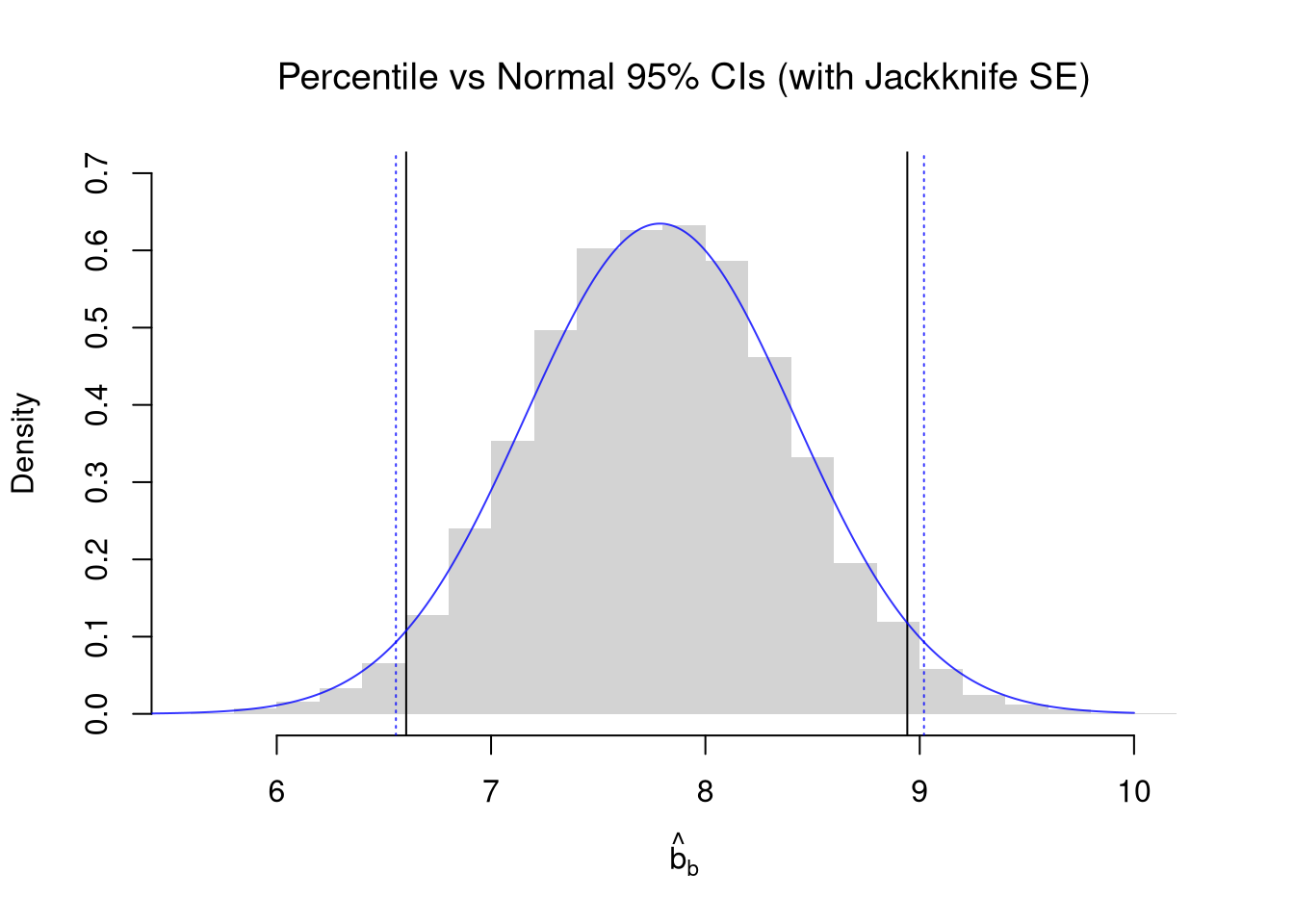
Note that you can also plug in Bootstrap or Jacknife SEs to the Normal Approximation.

## Bootstrap Distribution
hist(bootstrap_means, breaks=25,
    main=NA, border=NA,
    freq=F, ylim=c(0, 0.7),
    xlab=expression(hat(b)[b]))
abline(v=boot_ci_percentile, lty=1)
title('Percentile vs Normal 95% CIs (with Jackknife SE)', font.main=1)

# Jackknife SE Estimate
n <- length(sample_dat)
jackknife_means <- rep(NA, n)
for(i in seq_along(jackknife_means)){
    dat_noti <- sample_dat[-i]
    mean_noti <- mean(dat_noti)
    jackknife_means[i] <- mean_noti
}
se_jack <- sd(jackknife_means)*sqrt(n)

# Normal Approx with Jack SE
x <- seq(5, 10, by=0.01)
fx <- dnorm(x, sample_mean, se_jack)
lines(x, fx, col=rgb(0, 0, 1, .8), lty=1)
ci_normal_alt <- qnorm(c(.025, .975), sample_mean, se_jack)
abline(v=ci_normal_alt, col=rgb(0, 0, 1, .8), lty=3)

Update the example to use se_boot <- sd(bootstrap_means) in place of se_jack

7.3 Theoretical Properties

A \(Z\%\) confidence interval for the mean is an interval where \(Z\%\) of the intervals generated on different samples will contain the population mean \(\mu\).

n <- 30
B <- 100
sample_CIs <- matrix(nrow=B, ncol=2)
for(i in seq(1, B)){
    # Random Sample
    X <- runif(n)
    # Confidence Interval for each sample
    M <- mean(X)
    SE <- sd(X)/sqrt(n)
    CI <- qnorm( c(0.05, 0.95), M, SE)
    sample_CIs[i, ] <- CI
}


# Explicit calculation: whether the true mean is in each CI
mu_true <- 0.5 # theoretical result for uniform samples
covered <- mu_true >= sample_CIs[, 1] & mu_true <= sample_CIs[, 2]

# Visualize confidence intervals
plot.new()
plot.window(xlim = range(sample_CIs), ylim = c(0, B))
for(i in seq(1, B) ) {
  col_i <- if (covered[i]) rgb(0, 0, 0, 0.3) else rgb(1, 0, 0, 0.5)
  segments(
    sample_CIs[i, 1], i,
    sample_CIs[i, 2], i,
    col = col_i, lwd = 2)
}
abline(v = mu_true, col = rgb(0, 0, 1, .8), lwd = 2)
axis(1)
title('90% Coverage (Red = Missed)', font.main=1)

We typically have only one sample and compute a single confidence interval with the data we have. The interval you computed either contains the true mean or it does not.² So “\(Z\%\) confident” translates to “\(Z\%\) of intervals constructed on different samples will contain \(\mu\)”.

Sampling Distribution Quantiles.

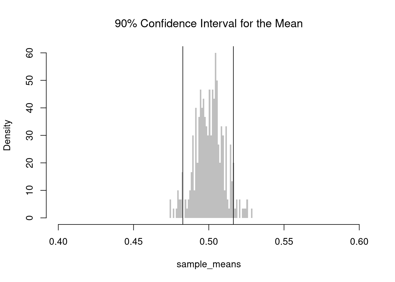
To better understand the link between our theoretical interpretation and our calculations, we will compute the quantiles of the sampling distribution. E.g., We construct a \(90\%\) confidence interval of the mean by taking the \(5^{th}\) and \(95^{th}\) percentiles of the sampling distribution of the mean. We conduct a simulation that shows the sampling distribution of the sample mean for a uniform random sample with a sample size of \(n=1000\), and then construct a confidence interval using quantiles.

# Create 300 samples, each with 1000 random uniform variables
X_samples <- matrix(nrow=300, ncol=1000)
for(i in seq(1, nrow(X_samples))){
    X_samples[i, ] <- runif(1000)
}
sample_means <- apply(X_samples, 1, mean) # mean for each sample (row)

# Middle 90%
mq <- quantile(sample_means, probs=c(.05, .95))
paste0('we are 90% confident that the mean is between ', 
    round(mq[1], 2), ' and ', round(mq[2], 2) )
## [1] "we are 90% confident that the mean is between 0.48 and 0.52"

hist(sample_means,
    breaks=seq(.4, .6, by=.001),
    border=NA, freq=F,
    col=rgb(0, 0, 0, .25),
    main=NA)
title('90% Confidence Interval for the Mean', font.main=1)
abline(v=mq)

TipTest Yourself

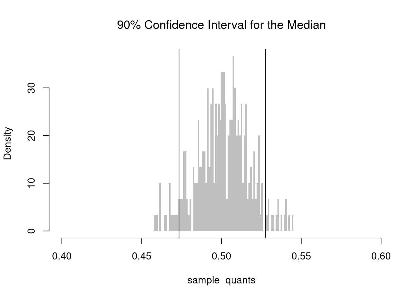
For another example, consider the median. We now repeat the above process to estimate the median for each sample, instead of the mean.

## Sample Quantiles (medians)
sample_quants <- apply(X_samples, 1, quantile, probs=0.5) #quantile for each sample (row)

# Middle 90% of estimates
mq <- quantile(sample_quants, probs=c(.05, .95))
paste0('we are 90% confident that the median is between ', 
    round(mq[1], 2), ' and ', round(mq[2], 2) )
## [1] "we are 90% confident that the median is between 0.47 and 0.52"

hist(sample_quants,
    breaks=seq(.4, .6, by=.001),
    border=NA, freq=F,
    col=rgb(0, 0, 0, .25),
    main=NA)
title('90% Confidence Interval for the Median', font.main=1)
abline(v=mq)

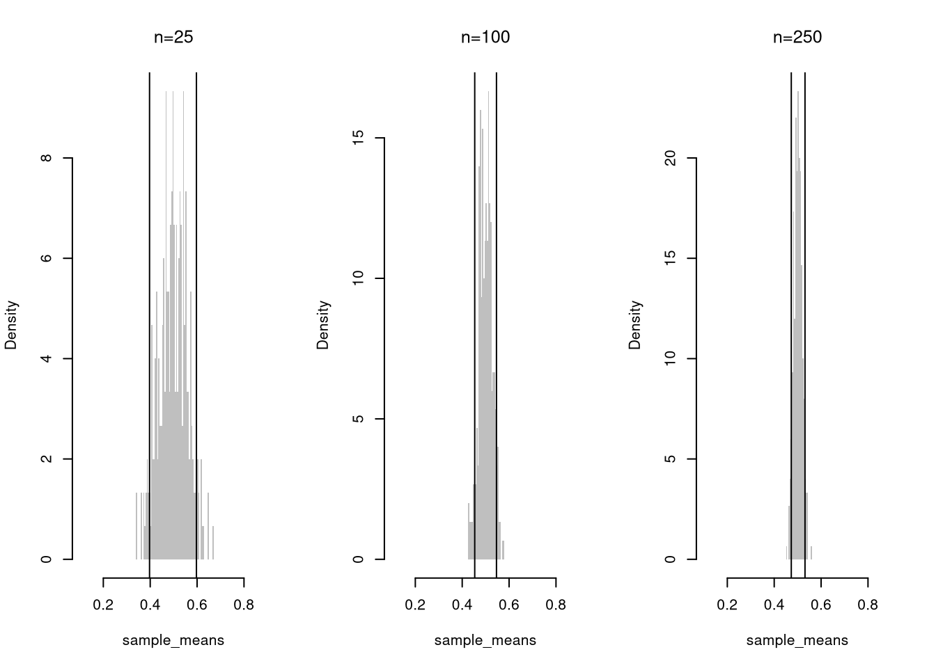
Interval Size.

Confidence intervals shrink with more data, as averaging washes out random fluctuations.

# Create 300 samples, each of size n
par(mfrow=c(1, 3))
for(n in c(25, 100, 250)){
    # Simulate 300 samples
    X_samples <- matrix(nrow=300, ncol=n)
    for(i in seq(1, nrow(X_samples))){
        X_samples[i, ] <- runif(n)
    }

    # Compute means for each sample (row)
    sample_means <- apply(X_samples, 1, mean)
    # 90% Confidence Interval
    mq <- quantile(sample_means, probs=c(.05, .95))
    hist(sample_means,
        breaks=seq(.1, .9, by=.005),
        border=NA, freq=F,
        col=rgb(0, 0, 0, .25),
        main=NA)
    title(paste0('n=', n), font.main=1)
    abline(v=mq)
}

Confidence intervals also shrink with lower probabilities of containing the theoretical value. For a fixed sample size \(n\), there is a trade-off between precision: the width of a confidence interval, and accuracy: the probability that a confidence interval contains the theoretical value.

TipTest Yourself

Here is an example showing what a Normal CI estimates. Theoretically, \(\pm 1 sd\) has 2/3 coverage. Change to \(\pm 2 sd\) to see Precision-Accuracy tradeoff.

# Normal CI for each sample
xq <- apply(X_samples, 1, function(r){ #theoretical se's
    mean(r) + c(-1, 1)*sd(r)/sqrt(length(r))
})
# First 3 interval estimates
xq[, c(1, 2, 3)]
##           [,1]      [,2]      [,3]
## [1,] 0.4462331 0.4979957 0.4817571
## [2,] 0.4833530 0.5336661 0.5182548

# Explicit calculation
mu_true <- 0.5 # theoretical result for uniform samples
# Logical vector: whether the true mean is in each CI
covered <- mu_true >= xq[1, ] & mu_true <= xq[2, ]
# Empirical coverage rate
coverage_rate <- mean(covered)
cat(sprintf('Estimated coverage probability: %.2f%%\n', 100 * coverage_rate))
## Estimated coverage probability: 65.67%

7.4 Misc. Topics

One-Sided Intervals.

Above, our confidence intervals were two-sided: they contained the middle \(Z\%\) of the sampling distribution. We can also construct one-sided intervals that extend to infinity in one direction.

A one-sided interval is shifted to one side, containing one tail rather than the middle. For example, an upper-bounded interval uses \((-\infty, q_{0.95}]\), where \(q_{0.95}\) is the \(95^{\text{th}}\) percentile of the bootstrap distribution: we are \(95\%\) confident the true value is at most \(q_{0.95}\). A lower-bounded interval uses \([q_{0.05}, \infty)\), where \(q_{0.05}\) is the \(5^{\text{th}}\) percentile of the bootstrap distribution: we are \(95\%\) confident the true value is at least \(q_{0.05}\).

NoteMust Know

For the electricity bill example above with \(\hat{M}=142\) and \(SE=5\), a one-sided \(95\%\) upper-bounded confidence interval is \[(-\infty,~ \hat{M} + 1.645 \times SE] = (-\infty,~ 142 + 1.645 \times 5] = (-\infty,~ 150.2].\] We are \(95\%\) confident the population mean bill is at most \(\$150.20\). Note that \(1.645\) is the \(95^{\text{th}}\) percentile of the standard normal (compared to \(1.96\) for the two-sided case).

M_hat <- 142
SE <- 5
# One-sided 95% upper bound
M_hat + qnorm(0.95) * SE
## [1] 150.2243

TipTest Yourself

Here is a bootstrap right-tail example

# Bootstrap Distribution
set.seed(1) # to be replicable
bootstrap_means <- rep(NA, 9999)
for(b in seq_along(bootstrap_means)){
    dat_id <- seq(1, length(sample_dat))
    boot_id <- sample(dat_id, replace=T)
    dat_b  <- sample_dat[boot_id] # c.f. jackknife
    mean_b <- mean(dat_b)
    bootstrap_means[b] <-mean_b
}

# One-sided 95% lower bound
# We are 95% confident the mean is at least q_05
hist(bootstrap_means, border=NA, breaks=50,
    freq=F, main=NA, xlab='Bootstrap')
abline(v=sample_mean, col=rgb(0, 0, 1, .8))
ci_95 <- quantile(bootstrap_means, probs=c(0.05, 1) )
abline(v=ci_95, lwd=2)

Prediction Intervals.

Note that \(Z\%\) confidence intervals do not generally cover \(Z\%\) of the data (those types of intervals are covered later). In the examples above, notice the confidence interval for the mean differs from the confidence interval of the median, and so both cannot cover \(90\%\) of the data. The confidence interval for the mean is roughly \([0.48, 0.52]\), which theoretically covers only a \(0.52-0.48=0.04\) proportion of uniform random data, much less than the proportion \(0.9\).

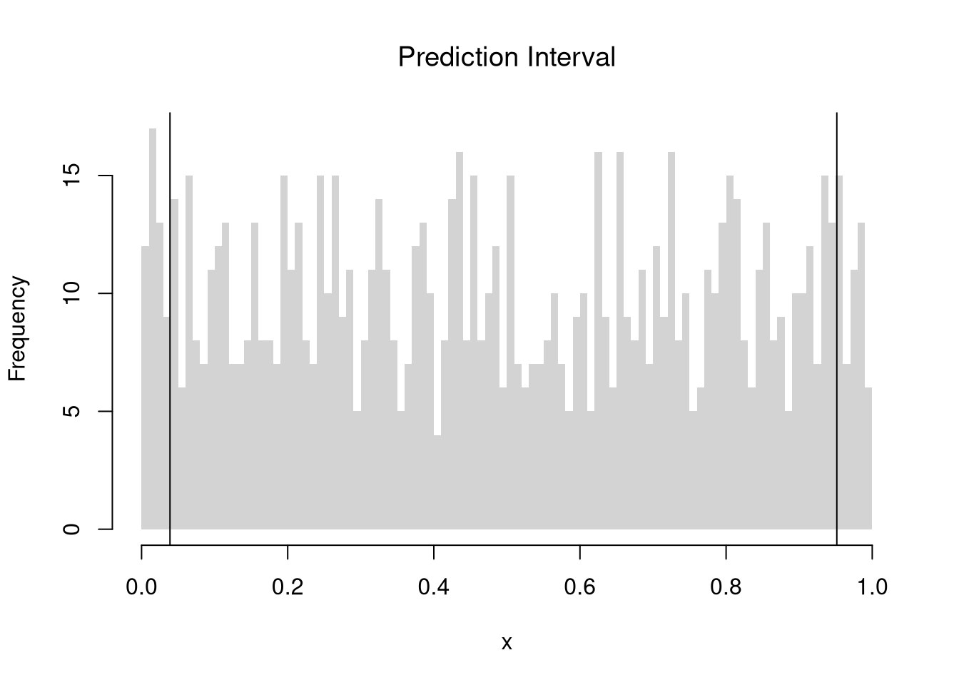
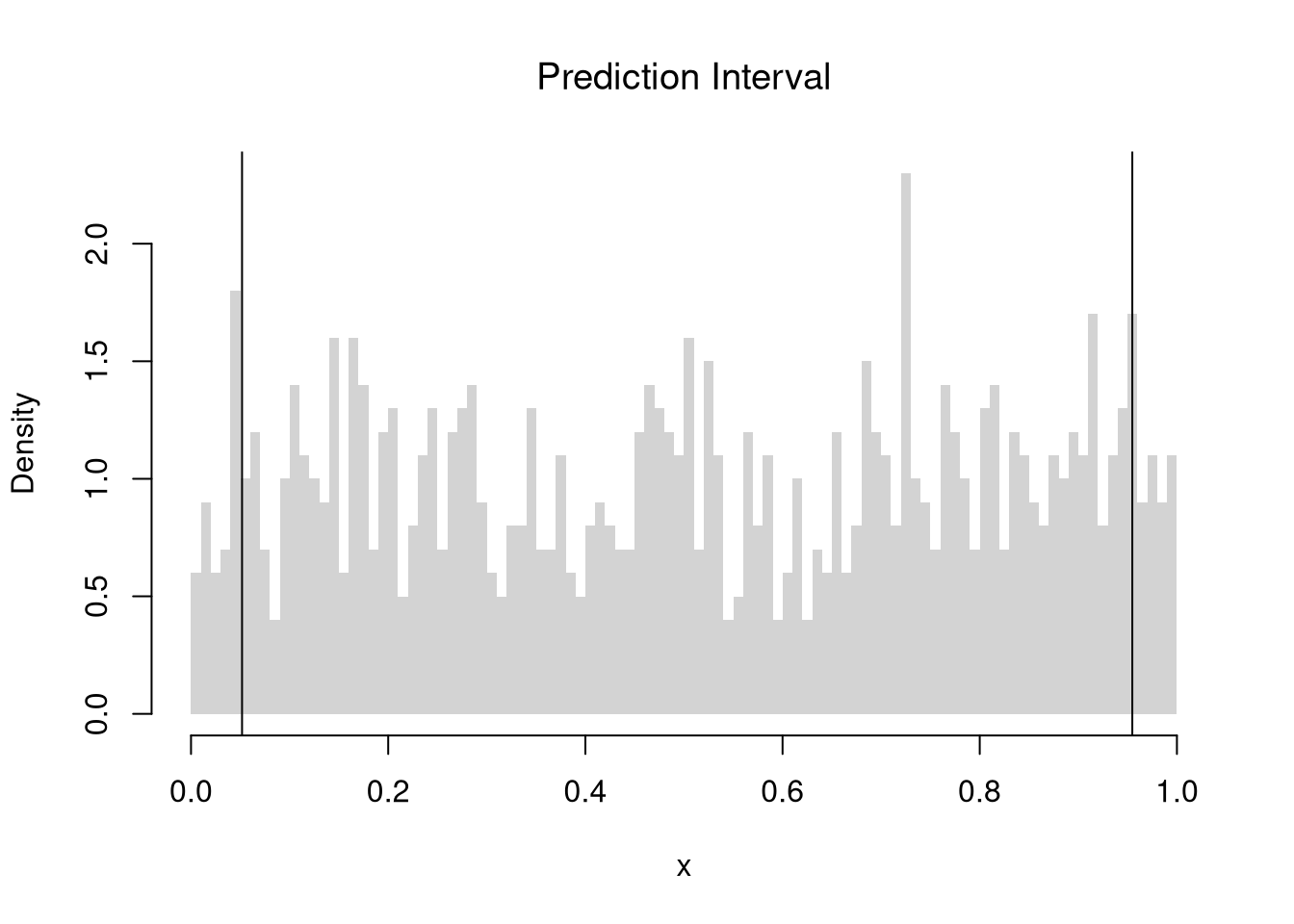
In addition to confidence intervals, we can also compute a prediction interval which estimate the variability of new data rather than a statistic. To do so, we compute the lower/upper quantiles of the data.

x <- runif(1000)
# Middle 90% of values
xq0 <- quantile(x, probs=c(.05, .95))
paste0('we are 90% confident that a future data point will be between ', 
    round(xq0[1], 2), ' and ', round(xq0[2], 2) )
## [1] "we are 90% confident that a future data point will be between 0.05 and 0.95"

hist(x,
    breaks=seq(0, 1, by=.01), border=NA,
    freq=F, main=NA)
title('Prediction Interval', font.main=1)
abline(v=xq0)

Confidence intervals also apply to regression coefficients. See Simple Regression for how these ideas extend to slopes and intercepts.

7.5 Exercises

1. A 95% confidence interval does not mean there is a 95% probability the true parameter lies inside that particular interval. Explain what “95% confident” actually means in terms of repeated sampling.

2. Suppose a sample of \(n = 49\) light bulbs has a mean lifetime of \(\hat{M} = 1200\) hours with a sample standard deviation of \(\hat{S} = 140\) hours. Compute the 90% and 99% Normal-approximation confidence intervals for the population mean lifetime. Which interval is wider, and why?

3. Using the USArrests dataset in R, construct a bootstrap 95% confidence interval for the median of the UrbanPop variable. Use at least 9999 bootstrap resamples and plot the bootstrap distribution with the interval boundaries.

Further Reading.

• https://learningstatisticswithr.com/book/estimation.html#interval-estimates – Confidence intervals explained with intuition and R code.
• https://www.khanacademy.org/math/statistics-probability/confidence-intervals-one-sample – Video walkthroughs of confidence interval construction and interpretation.
• https://www.econometrics-with-r.org/3.1-hypothesis-tests-and-confidence-intervals-in-the-simple-linear-regression-model.html – Confidence intervals applied to regression, bridging descriptive and inferential statistics.

---

1. Generally, a coverage level of \(1-\alpha\) means \(Prob( M - E < \mu < M + E)=1-\alpha\). Notice that \(Prob( M - E < \mu < M + E) = Prob( - E < \mu - M < + E) = Prob( \mu + E > M > \mu - E)\). So if the interval \([\mu - 10, \mu + 10]\) contains \(95\%\) of all \(M\), then the interval \([M-10, M+10]\) will also contain \(\mu\) in \(95\%\) of the samples because whenever \(M\) is within \(10\) of \(\mu\), the value \(\mu\) is also within \(10\) of \(M\). But for any particular sample, the interval \([\hat{M}-10, \hat{M}+10]\) either does or does not contain \(\mu\). Similarly, if you compute \(\hat{M}=9\) for your particular sample, a coverage level of \(1-\alpha=95\%\) does not mean \(Prob(9 - E < \mu < 9 + E)=95\%\).

2. As such, a \(Z\%\) confidence interval does not imply a \(Z\%\) probability that the true parameter lies within a particular calculated interval. In practice, people often interpret confidence intervals informally as “showing the uncertainty around our estimate”: wider intervals correspond to higher sampling variability and less precise information about \(\mu\).