Code
## Minimal example
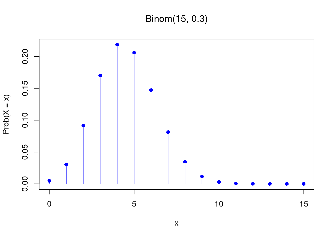
n <- 15
p <- 0.3
# PMF plot
x <- seq(0, n)
f_x <- dbinom(x, n, p)
plot(x, f_x, type = "h", col = "blue",
main='', xlab = "x", ylab = "Prob(X = x)")
title(bquote(paste('Binom(',.(n),', ',.(p), ')' ) ))
points(x, f_x, pch = 16, col = "blue")
Code
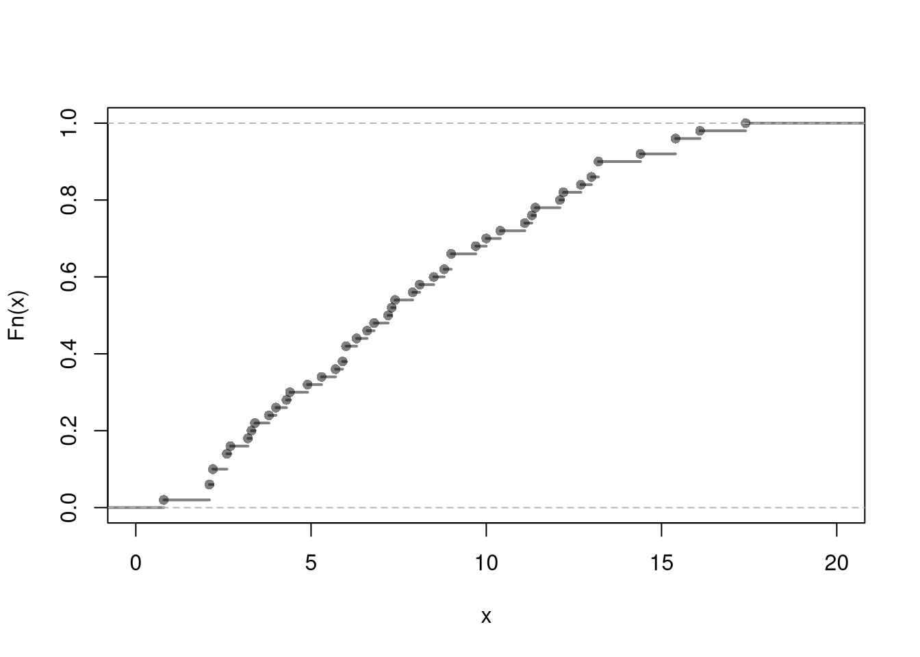
## Simulation
X <- rbinom(1000, n, p)
plot(ecdf(X))