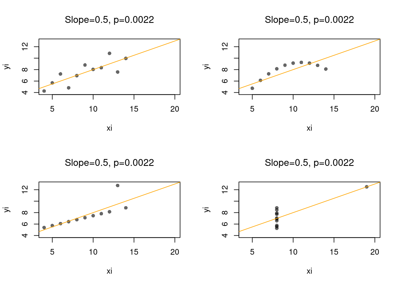
Scatterplots are a great and simplest plot for bivariate data that simply plots each observation. There are many extensions and similar tools. The example below helps understand how both the central tendency and dispersion change.
Code
# Local relationship: wages and educationlibrary(wooldridge)## Plot 1plot(wage~educ, data=wage1, pch=16, col=grey(0,.1))educ_means <-aggregate(wage1[,c("wage","educ")],list(wage1[,'educ']), mean)points(wage~educ, data=educ_means, pch=17, col='blue', type='b')title("Grouped Means and Scatterplot", font.main=1)
Code
## Plot 2 (Alternative for big datasets)# boxplot(wage~educ, data=wage1, # pch=16, col=grey(0,.1), varwidth=T)#title("Boxplots", font.main=1)## Plot 3 (Less informative!)#barplot(wage~educ, data=educ_means)#title("Bar Plot of Grouped Means", font.main=1)
Note
Examine the local relationship between ‘Murder’ and ‘Urbanization’ in the USArrests dataset.
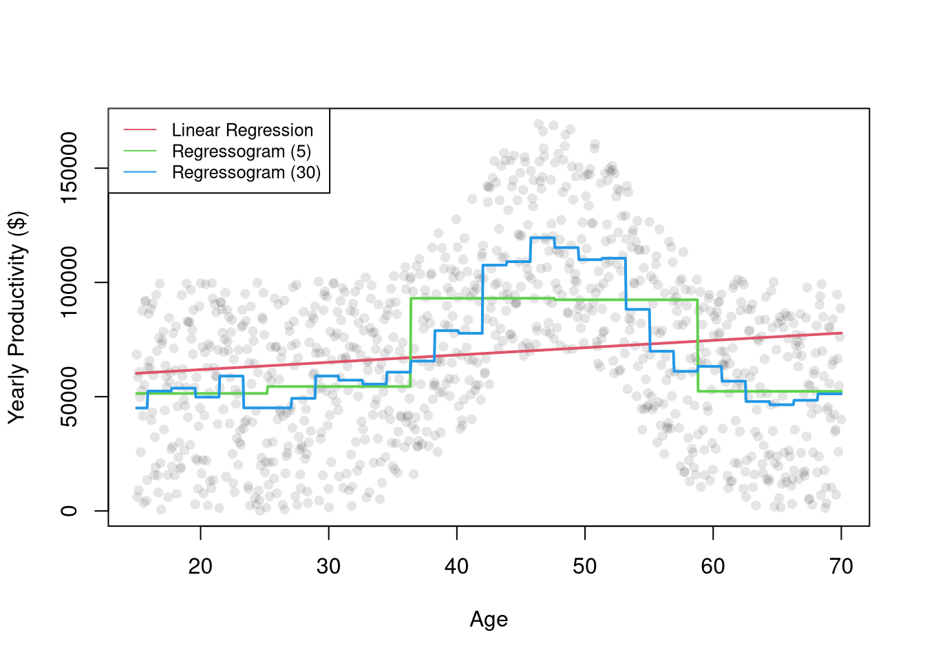
Just as we use histograms to describe the distribution of a random variable, we can use a regressogram for conditional relationships. Specifically, we can use dummies for exclusive intervals or bins to estimate how the average value of \(Y\) varies with \(X\).
After dividing \(X\) into \(1,...L\) exclusive bins of width \(h\). Each bin has a midpoint, \(x\), and an associated dummy variable \(\hat{D}_{i}(x,h) = \mathbf{1}\left(\hat{X}_{i} \in \left(x-h/2,x+h/2\right] \right)\).1 Then conduct a dummy variable regression \[\begin{eqnarray}
\hat{Y}_{i} &=& \sum_{x \in \{x_{1}, ..., x_{L} \}} b_{0}(x,h) \hat{D}_{i}(x,h) + e_{i},
\end{eqnarray}\] where each bin has a coefficient \(b_{0}(x,h)\).
Consider this two-bin example of how age affects wage for people with \(\leq 10\) years of school complete vs \(> 10\). \[\begin{eqnarray}
\text{Wage}_{i} &=& b_{0}(x=5, h=10) \mathbf{1}\left(\text{Educ}_{i} \in [0,10]\right) + b_{0}(x=15, h=10) \mathbf{1}\left(\text{Age}_{i} \in (10,20] \right) + e_{i}.
\end{eqnarray}\] You could also look at three bins to see if that is a better fit. You can also try finer bins and see what grouping emerges naturally (e.g., whether the main effect on wages is whether your not in school or retired).
Notice that each bin has \(n(x,h) = \sum_{i}^{n}\hat{D}_{i}(x,h)\) observations. This means we can split the dataset into parts associated with each bin \[\begin{eqnarray}
\label{eqn:regressogram1}
\sum_{i}^{n}\left[e_{i}\right]^2
&=& \sum_{i}^{n}\left[\hat{Y}_{i}- \sum_{x \in \{x_{1}, ..., x_{L} \}} b_{0}(x,h) \hat{D}_{i}(x,h) \right]^2 \\
&=& \sum_{i}^{n(x_{1},h)}\left[\hat{Y}_{i}- \sum_{x \in \{x_{1}, ..., x_{L} \}} b_{0}(x,h) \hat{D}_{i}(x,h) \right]^2 + ... \nonumber \\
& & \sum_{i}^{n(x_{L},h)}\left[\hat{Y}_{i}- \sum_{x \in \{x_{1}, ..., x_{L} \}} b_{0}(x,h) \hat{D}_{i}(x,h) \right]^2 \\
&=& \sum_{i}^{n(x_{1},h)}\left[\hat{Y}_{i}- b_{0}\left(x_1,h\right) \right]^2 + ... \sum_{i}^{n(x_L,h)}\left[\hat{Y}_{i}-b_{0}\left(x_L,h\right) \right]^2 % +~ (N-1)\sum_{i}\hat{Y}_{i}.
\end{eqnarray}\] This separation allows us optimize for each bin separately \[\begin{eqnarray}
\label{eqn:regressogram2}
\min_{ \left\{ b_{0}(x,h) \right\} } \sum_{i}^{n}\left[e_{i}\right]^2
&=& \min_{ \left\{ b_{0}(x,h) \right\} } \sum_{i}^{n(x,h)}\left[\hat{Y}_{i}- b_{0}\left(x,h\right) \right]^2,
\end{eqnarray}\] since, in either case, minimizing yields \[\begin{eqnarray}
0 &=& -2 \sum_{i}^{n(x,h)}\left[ \hat{Y}_{i} - b_{0}(x,h) \right] \\
\hat{b}_{0}(x,h) &=& \frac{\sum_{i}^{n(x,h)} \hat{Y}_{i}}{ n(x,h) } = \hat{M}_{Y}(x,h) .
\end{eqnarray}\] As such, the OLS regression yields coefficients that are interpreted as the conditional mean: \(\hat{M}_{Y}(x,h)\). We can directly compute the same statistic directly by simply takes the average value of \(\hat{Y}_{i}\) for all \(i\) observations in a particular bin. The values predicted by the model are then found as \(\hat{y}_{i} = \sum_{x} \hat{b}_{0}(x,h) \hat{D}_{i}(x,h)\).
Interestingly, we can obtain the same statistic from weighted least squares regression. For some specific design point, \(x\), we can find \(\hat{b}(x, h)\) by minimizing \[\begin{eqnarray}
\sum_{i}^{n}\left[ e_{i} \right]^2 \hat{D}_{i}(x,h) &=& \sum_{i}^{n}\left[ \hat{Y}_{i}- b_{0}(x,h) \right]^2 \hat{D}_{i}(x,h) \\
&=& \sum_{i}^{n(x_{1},h)}\left[ \hat{Y}_{i}- b_{0}(x_{1},h) \right]^2 \hat{D}_{i}(x_{1},h) + ... \sum_{i}^{n(x_{L},h)}\left[ \hat{Y}_{i}- b_{0}(x_{L},h) \right]^2 \hat{D}_{i}(x_{L},h) \\
&=& \sum_{i}^{n(x,h)}\left[\hat{Y}_{i}- b_{0}\left(x,h\right) \right]^2
\end{eqnarray}\]
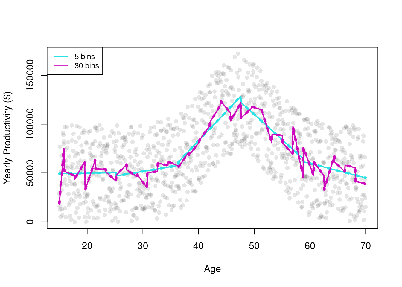
Piecewise Regression.
The regressogram depicts locally constant relationships. We can also included slope terms within each bin to allow for locally linear relationships. This is often called segmented/piecewise regression, which runs a separate regression for different subsets of the data.
# See that two methods give the same predictions## Course Age Binspred2 <-predict(reg2)## Split Sample Regressionsdat2 <-split( dat, dat[,'xcc'])pred2B <-lapply(dat2, function(d){ reg2 <-lm(wage~educ, d) pred_d <-predict(reg2)})# Any differences?all( pred2 -unlist(pred2B) <1e-10 )## [1] FALSE
Note
Compare a simple regression to a regressogram and a piecewise regression. Examine the relationship between ‘Murder’ and ‘Urbanization’ in the USArrests dataset.
For many things, a simple linear regression, regressograms, or piecewise regression is “good enough”. Simple linear regressions struggle with nonlinear relationships but are very easy to run with a computer. Regressograms and piecewise regressions are intuitive ways to capture nonlinear relationships that are computationally efficient but have obvious problems where the bins change. Sometimes we want smoother predictions or to estimate derivatives (gradients). To cover more advanced regression methods that do those things, we will need to first learn about kernel density estimation.
14.2 Kernel Density Estimation
A kernel density is generally a “smooth” version of a histogram. We estimate the density at many points (e.g., all unique values \(x\) in the dataset), not just the midpoints of exclusive bins. The uniform kernel and density estimator is \[\begin{eqnarray}
\label{eqn:uniform}
\hat{f}_{U}(x) &=& \frac{1}{n} \sum_{i}^{n} \frac{k_{U}(\hat{X}_{i}, x, h) }{2h} \\
k_{U}\left( \hat{X}_{i}, x, h \right) &=& \mathbf{1}\left(\frac{|\hat{X}_{i}-x|}{h}<1\right)
= \mathbf{1}\left( \hat{X}_{i} \in \left( x-h, x + h\right) \right).
\end{eqnarray}\] Notice that the uniform kernel is essentially the histogram but without the restriction that \(x\) must be a midpoint of exclusive bins. Typically, the points \(x\) are chosen to be either the unique observations or some equidistant set of “design points”.
We can also replace the uniform kernel with a more general kernel function \(k\), which is then normalized to an easier to read and program \(K\) function: \(k\left( \hat{X}_{i}, x, h \right)= K\left( \frac{|\hat{X}_{i}-x|}{h} \right)\). We can then define a general kernel function as a non-negative real-valued function \(K\) that integrates to unity: \[\begin{eqnarray}
\int_{-\infty}^{\infty} K(v) dv &=& 1
\end{eqnarray}\] The general idea behind kernel density is to use windows around each \(x\) that potentially overlap, rather than partitioning the range of \(X\) into exclusive bins.2 There are many kernels, but these are the most intuitive and commonly used.
Code
# Kernel Density FunctionsX <-seq(-2,2, length.out=1001)plot.new()plot.window(xlim=c(-1.2,1.2), ylim=c(0,1))h <-1lines( dunif(X,-h,h)~X, col=1, lty=1)h <-1/2lines( dnorm(X,0,h)~X, col=2, lty=1)dtricub <-function(X, x=0, h){ u <-abs(X-x)/h fu <-70/81*(1-u^3)^3/h*(u <=1)return(fu)}h <-1lines( dtricub(X,0,h)~X, col=3, lty=1)h <-1/2lines(density(x=0, bw=h, kernel="epanechnikov"), col=4, lty=1)## Note that "density" defines h slightly differentlyrug(0, lwd=2)axis(1)axis(2)legend('topright', lty=1, col=1:4,legend=c('uniform(1)', 'gaussian(1/2)', 'tricubic(1)', 'epanechnikov(1)'))
Once we have picked a kernel (which particular one is not particularly important) we can use it to compute density estimates at each design point.
Code
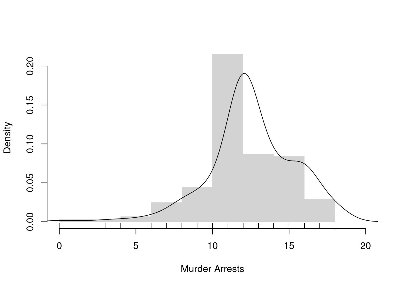
# Practical ExampleX <- wage1[,'educ']hist(X,breaks=seq(0,20,by=2), #bin width=1freq=F,border=NA, main='',xlab='Murder Arrests')# Density Estimatelines(density(X, bw=1))# Raw Observationsrug(wage1[,'educ'], col=grey(0,.5))
Note
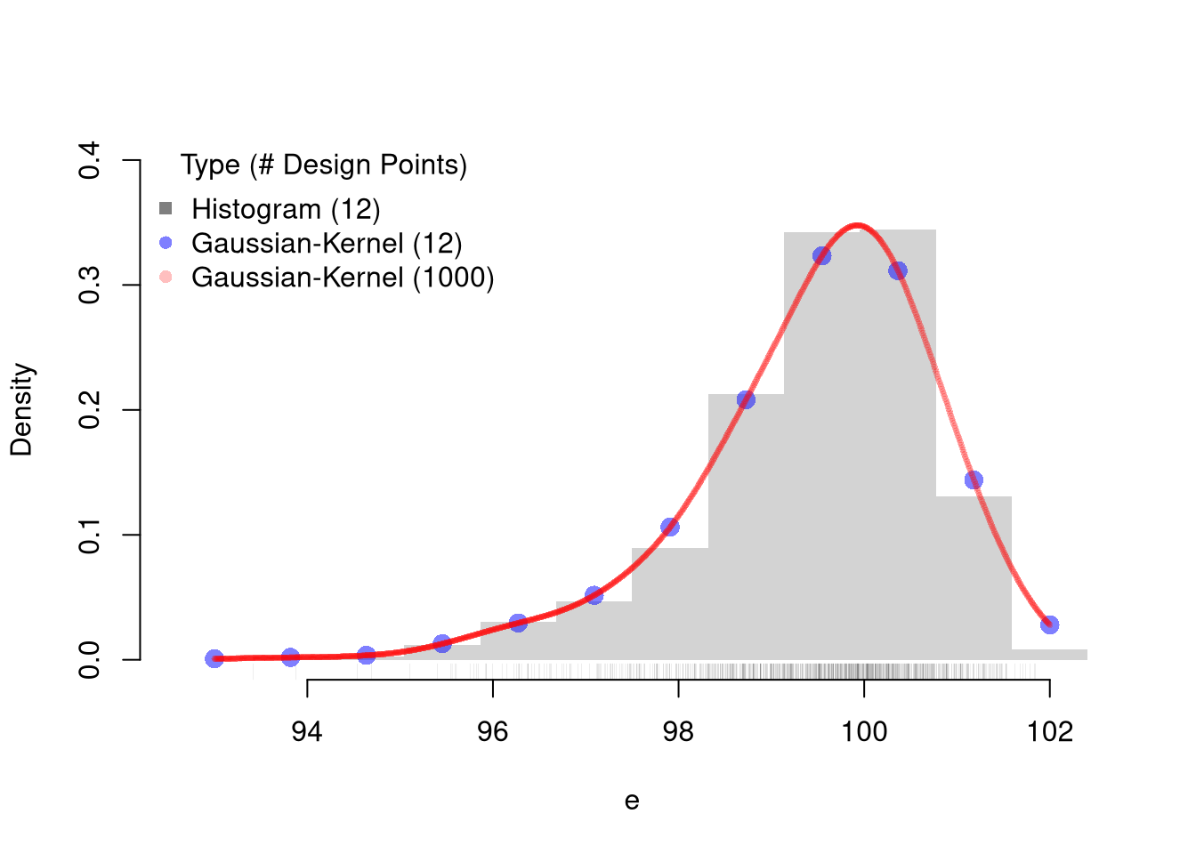
Here is an example going into the details of KDE.
Code
# Kernel Density EstimationN <-1000e <-rweibull(N,100,100)ebins <-seq(floor(min(e)), ceiling(max(e)), length.out=12)## Histogram Estimates at 12 pointsxbks <-c(ebins[1]-diff(ebins)[1]/2, ebins+diff(ebins)[1]/2)hist(e, freq=F, main='', breaks=xbks, ylim=c(0,.4), border=NA)rug(e, lwd=.07, col=grey(0,.5)) ## Sample## Manually Compute Uniform Estimate at X=100 with h=2# w100 <- (e < 101)*(e > 99)# sum(w100)/(N*2)## Gaussian Estimates at same points as histogramF_hat <-sapply(ebins, function(x,h=.5){ kx <-dnorm( abs(e-x)/h ) fx <-sum(kx,na.rm=T)/(h*N) fx})## Verify the samefhat1 <-density(e, n=12, from=min(ebins), to=max(ebins), bw=.5)points(fhat1[['x']], fhat1[['y']], pch=16, col=rgb(0,0,1,.5), cex=1.5)## Gaussian Estimates at all sample pointsfhat2 <-density(e, n=1000, from=min(ebins), to=max(ebins), bw=.5)points(fhat2[['x']], fhat2[['y']], pch=16, col=rgb(1,0,0,.25), cex=.5)legend('topleft', pch=c(15,16,16),col=c(grey(0,.5),rgb(0,0,1,.5), rgb(1,0,0,.25)),title='Type (# Design Points)', bty='n',legend=c('Histogram (12)','Gaussian-Kernel (12)','Gaussian-Kernel (1000)'))
14.3 Local Linear Regression
It is safer to assume that you could be analyzing data with nonlinear relationships. A general nonparametric model is written as \[\begin{eqnarray}
\hat{Y}_{i} = m(\hat{X}_{i}) + \epsilon_{i}
\end{eqnarray}\] where \(m\) is an unknown continuous function and \(\epsilon\) is white noise. (As such, the linear model is a special case.) You can estimate the mean of \(Y_{i}\) conditional on \(X_{i}=x\) with a regressogram or a variety of other least-squares procedures.
Locally Constant (Moving Average).
Consider a point \(x\) and suppose \(\hat{Y}_{i} = b(x,h) + e_{i}\) locally. Then notice a weighted OLS estimator with uniform kernel weights yields \[\begin{eqnarray} \label{eqn:lcls}
& & \min_{b(x,h)}~ \sum_{i}^{n}\left[e_{i} \right]^2 k_{U}\left( \hat{X}_{i}, x, h \right) \\
\Rightarrow & & -2 \sum_{i}^{n}\left[\hat{Y}_{i}- b(x,h) \right] k_{U}\left(\hat{X}_{i}, x, h\right) = 0\\
\label{eqn:lcls1}
\Rightarrow & & \hat{b}_{U}(x)
= \frac{\sum_{i} \hat{Y}_{i} k_{U} \left( \hat{X}_{i}, x, h \right) }{ \sum_{i} k_{U}\left( \hat{X}_{i}, x, h \right) }
= \sum_{i} \hat{Y}_{i} \left[ \frac{ k_{U} \left( \hat{X}_{i}, x, h \right) }{ \sum_{i} k_{U}\left( \hat{X}_{i}, x, h \right)} \right] = \sum_{i} \hat{Y}_{i} w_{i},
\end{eqnarray}\] where weight \(w_{i} = \mathbf{1}\left( |\hat{X}_{i} - x| < h \right)/N\) because \(k_{U} \left( \hat{X}_{i}, x, h \right)\) is either one or zero, and \(\sum_{i} k_{U} \left( \hat{X}_{i}, x, h \right) = n(x,h)\). So locally constant kernel regression recovers the weighted mean of \(Y_{i}\) around design point \(x\). If we use exclusive bins, then we are running a regressogram, which is more crude but can be estimated easily.
When \(n\) is small, \(\hat{b}_{U}(x)\) is typically estimated for each unique observed value: \(x \in \{ x_{1},...x_{n} \}\). For large datasets, you can select a subset or evenly spaced values of \(x\) for which to estimate \(\hat{b}_{U}(x)\).
Note
Here is an example going into the details of LCLS.
The basic idea also generalizes other kernels. As such, a kernel regression using uniform weights is often called a “naive kernel regression”. Typically, kernel regressions use kernels that weight nearby observations more heavily. We can also add a slope term to improve the fit.
If \(X_{i}\) represents time, then the local constant regressions is also called a moving average. With non-uniform kernel weights, we have a weighted moving average.
Locally Linear.
A less simple case is a local linear regression which conducts a linear regression for each data point using a subsample of data around it. Consider a point \(x\) and suppose \(\hat{Y}_{i} = b_{0}(x,h) + b_{1}(x) \hat{X}_{i} + e_{i}\) for data near \(x\). The weighted OLS estimator with kernel weights is \[\begin{eqnarray}
& & \min_{b_{0}(x,h),b_{1}(x,h)}~ \sum_{i}^{n}\left[\hat{Y}_{i}- b_{0}(x,h) - b_{1}(x,h) \hat{X}_{i} \right]^2 K\left(\frac{|\hat{X}_{i}-x|}{h}\right)
\end{eqnarray}\] Deriving the optimal values \(\hat{b}_{0}(x,h)\) and \(\hat{b}_{1}(x,h)\) for \(k_{U}\) is left as a homework exercise.3
Code
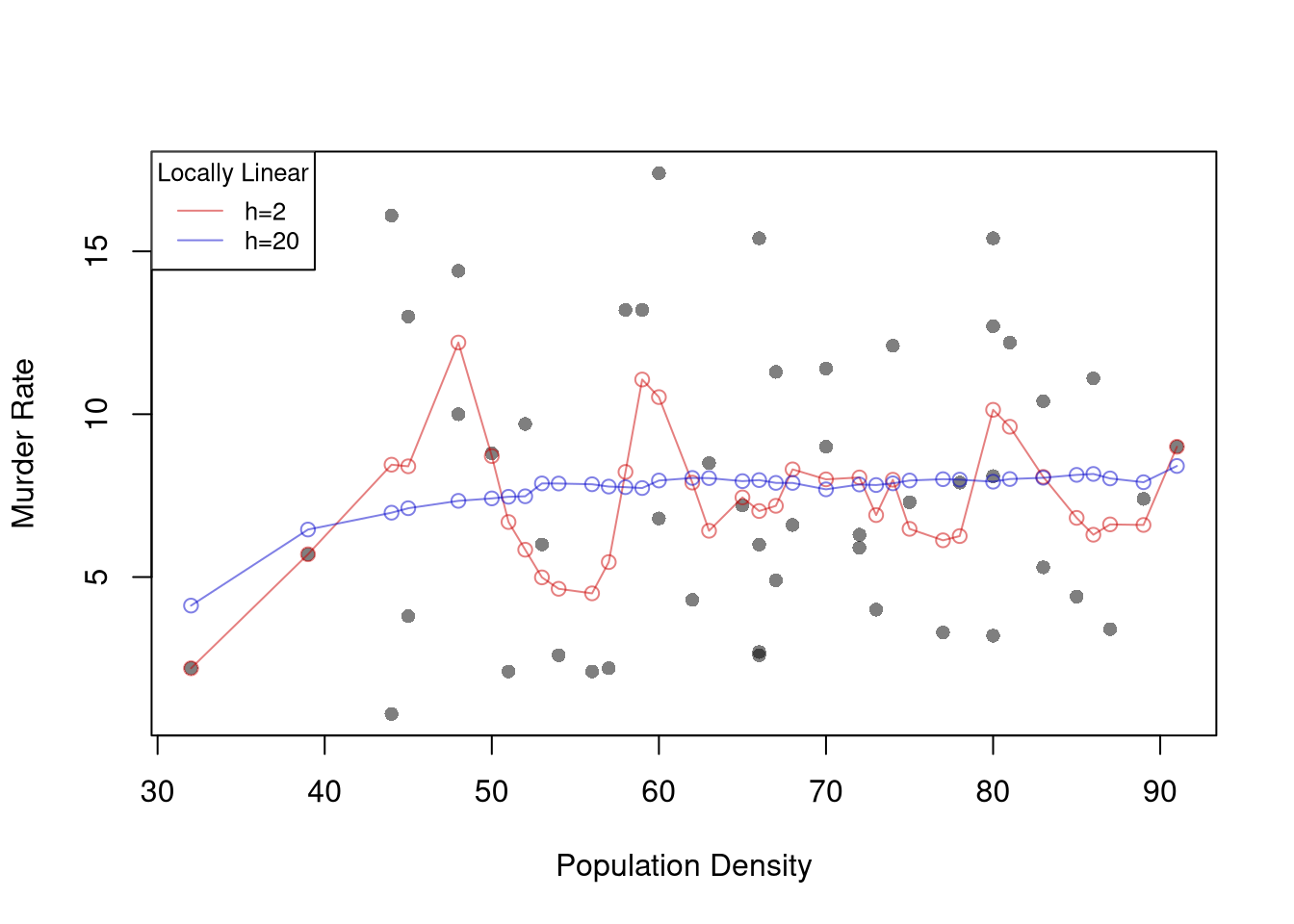
# ``Naive" Smootherpred_fun <-function(x0, h, xy){# Assign equal weight to observations within h distance to x0# 0 weight for all other observations ki <-dunif(xy[,'x'], x0-h, x0+h) llls <-lm(y~x, data=xy, weights=ki) yhat_i <-predict(llls, newdata=data.frame(x=x0))}xy <- wage1[,c('educ','wage')]names(xy) <-c('x','y')X0 <-sort(unique(xy[,'x']))pred_lo1 <-sapply(X0, pred_fun, h=2, xy=xy)pred_lo2 <-sapply(X0, pred_fun, h=12, xy=xy)plot(wage~educ, pch=16, data=wage1, col=grey(0,.1),ylab='Murder Rate', xlab='Population Density')cols <-c(rgb(.8,0,0,.5), rgb(0,0,.8,.5))lines(X0, pred_lo1, col=cols[1], lwd=1, type='o')lines(X0, pred_lo2, col=cols[2], lwd=1, type='o')legend('topleft', title='Locally Linear',legend=c('h=2 ', 'h=12'),lty=1, col=cols, cex=.8)
Note
Compare local linear and local constant regressions using https://shinyserv.es/shiny/kreg/, with degree \(0\) and \(1\). Also try different kernels and different datasets.
Tip
Examine the local relationship between ‘Murder’ and ‘Urbanization’ in the USArrests dataset using LLLS with a Gaussian kernel.
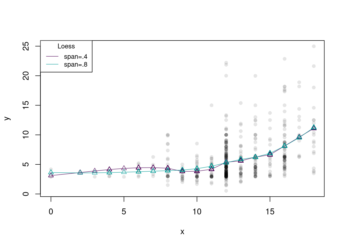
An important extension of locally linear regressions is called loess, which uses adaptive bandwidths in order to have a similar number of data points around each design point. This is especially useful when \(X\) is not uniform.
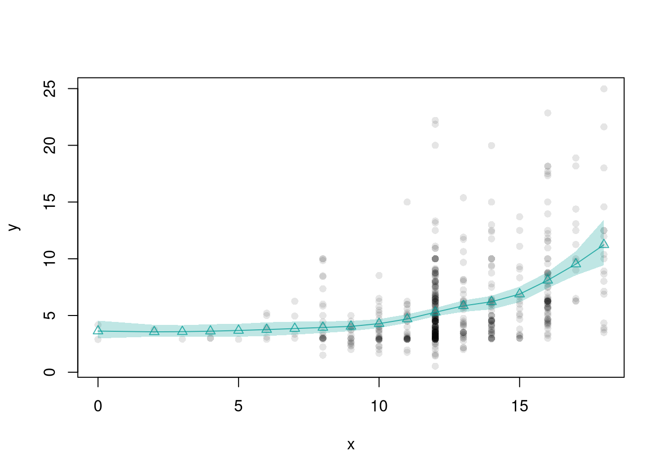
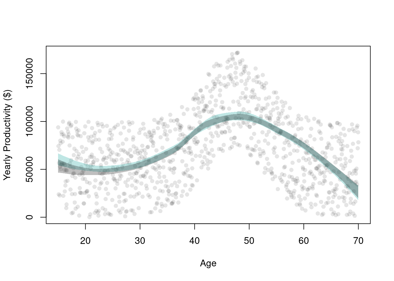
These confidence bands are approximations to what we want: how much do the predicted values vary from sample to sample. To make that clear, we will use a simulation where we can actually generate different samples.
Code
## AgesXmx <-70Xmn <-15##Generate Sample Datadat_sim <-function(n=1000){ n <-1000 X <-seq(Xmn,Xmx,length.out=n)## Random Productivity e <-runif(n, 0, 1E6) beta <-1E-10*exp(1.4*X -.015*X^2) Y <- (beta*X + e)/10return(data.frame(Y,X))}dat <-dat_sim(1000)## Data from one sampleplot(Y~X, data=dat, pch=16, col=grey(0,.1),ylab='Yearly Productivity ($)', xlab='Age' )dat0 <- dat[order(dat[,'X']),]reg_lo <-loess(Y~X, data=dat0, span=.8)## Plot Bootstrap CI for Single Samplepred_design <-data.frame(X=seq(Xmn, Xmx))preds_lo <-predict(reg_lo, newdata=pred_design)boot_lo <-sapply(1:399, function(b){ dat0_i <- dat0[sample(nrow(dat0), replace=T),] reg_i <-loess(Y~X, dat=dat0_i, span=.8)predict(reg_i, newdata=pred_design)})boot_cb <-apply(boot_lo,1, quantile,probs=c(.025,.975), na.rm=T)polygon(c(pred_design[[1]], rev(pred_design[[1]])),c(boot_cb[1,], rev(boot_cb[2,])),col=hcl.colors(3,alpha=.25)[2],border=NA)# Construct CI across Multiple Samplessample_lo <-sapply(1:399, function(b){ xy_b <-dat_sim(1000) #Entirely new sample reg_b <-loess(Y~X, dat=xy_b, span=.8)predict(reg_b, newdata=pred_design)})ci_lo <-apply(sample_lo,1, quantile,probs=c(.025,.975), na.rm=T)polygon(c(pred_design[[1]], rev(pred_design[[1]])),c(ci_lo[1,], rev(ci_lo[2,])),col=grey(0,alpha=.25),border=NA)
The bins do not all need to have the same width, but that is a good default and more notationally convenient than letting the bandwidth depend on the bin; \(h(x)\).↩︎
We only examine symmetric kernels, as some texts also include symmetric in the definition of a kernel; \(K(v) = K(-v)\).↩︎
Note that one general benefit of LLLS is with edge effects (see homework). Another is that it is theoretically motivated: assuming that \(Y_{i}=m(X_{i}) + \epsilon_{i}\), we can then take a Taylor approximation: \(m(X_{i}) + \epsilon_{i} \approx m(x) + m'(x)[X_{i}-x] + \epsilon_{i} = [m(x) - m'(x)x ] + m'(x)X_{i} + \epsilon_{i} = b_{0}(x,h) + b_{1}(x,h) X_{i}\). As such, a third benefit is that the estimated slope coefficient \(\hat{b}_{1}(x,h)\) can be interpreted as the estimated gradient at \(x\).↩︎