Code
# Bivariate Data from USArrests
xy <- USArrests[,c('Murder','UrbanPop')]
xy[1,]
##         Murder UrbanPop
## Alabama 13.2 58We will now study two variables. The data for each observation data can be grouped together as a vector \((\hat{X}_{i}, \hat{Y}_{i})\).
# Bivariate Data from USArrests
xy <- USArrests[,c('Murder','UrbanPop')]
xy[1,]
## Murder UrbanPop
## Alabama 13.2 58We have multiple observations of \((\hat{X}_{i}, \hat{Y}_{i})\), each of which corresponds to a unique value \((x,y)\). A frequency table shows how often each combination of values appear. The joint distribution counts up the number of pairs with the same values and divides by the number of obersvations, \(n\); \[\begin{eqnarray} \hat{p}_{xy} = \sum_{i=1}^{n}\mathbf{1}\left( \hat{X}_{i}=x, \hat{Y}_{i}=y \right)/n, \end{eqnarray}\] The marginal distributions are just the univariate information, which can be computed independantly as in https://jadamso.github.io/Rbooks/01_06_PopStatistics.html#estimates or from the joint distribution \[\begin{eqnarray} \hat{p}_{x} = \sum_{y} \hat{p}_{xy} \end{eqnarray}\]
For example, suppose we observe a sample of \(n=13\) students with two discrete variables:
Assume the count data are summarized by the following table:
\[\begin{array}{c|cc|c} & y=0\ (\text{male}) & y=1\ (\text{female})\\ \hline x=12 & 4 & 3 \\ x=14 & 1 & 5 \\ \hline \end{array}\] The joint distributions divides each cell count by the total number of observations to obtain \[\begin{array}{c|cc} & y=0 & y=1\\ \hline x=12 & 4/13 & 3/13 \\ x=14 & 1/13 & 5/13 \end{array}\]The marginal distribution of \(X_{i}\) is \[\begin{eqnarray} \hat{p}_{x=12} &=& \frac{4}{13} + \frac{3}{13} = \frac{7}{13},\\ \hat{p}_{x=14} &=& \frac{1}{13} + \frac{5}{13} = \frac{6}{13}. \end{eqnarray}\] The marginal distribution of \(Y_{i}\) is \[\begin{eqnarray} \hat{p}_{y=0} &=& \frac{4}{13} + \frac{1}{13} = \frac{5}{13} \approx 0.38,\\ \hat{p}_{y=1} &=& \frac{3}{13} + \frac{5}{13} = \frac{8}{13} \approx 0.62. \end{eqnarray}\]
Together, this yields a frequency table with marginals \[\begin{array}{c|cc|c} & y=0\ (\text{male}) & y=1\ (\text{female}) & \text{Row total}\\ \hline x=12 & 4/13 & 3/13 & 7/13\\ x=14 & 1/13 & 5/13 & 6/13\\ \hline \text{Column total} & 5/13 & 8/13 & 1 \end{array}\]# Simple hand-built dataset: 13 students
X <- c(rep(12,7), rep(14,6))
Y <- c(rep(0,4), rep(1,3), # among X=12: 4 male, 2 female
rep(0,1), rep(1,5)) # among X=14: 1 male, 5 female
dat <- data.frame(educ=X, female=Y)
# Frequency table
tab <- table(dat) # counts
prop <- tab/sum(tab) # joint distribution p_xy
round(prop, 2)
## female
## educ 0 1
## 12 0.31 0.23
## 14 0.08 0.38
# marginals directly
margin.table(prop, 1) # p_x
## educ
## 12 14
## 0.5384615 0.4615385
margin.table(prop, 2) # p_y
## female
## 0 1
## 0.3846154 0.6153846
# joint distribution with marginals added
addmargins(prop)
## female
## educ 0 1 Sum
## 12 0.30769231 0.23076923 0.53846154
## 14 0.07692308 0.38461538 0.46153846
## Sum 0.38461538 0.61538462 1.00000000Scatterplots are used frequently to summarizes the joint distribution of continuous data. They can be enhanced in several ways. As a default, use semi-transparent points so as not to hide any points (and perhaps see if your observations are concentrated anywhere). You can also add other features that help summarize the relationship, although I will defer this until later.
plot(Murder~UrbanPop, USArrests, pch=16, col=grey(0.,.5))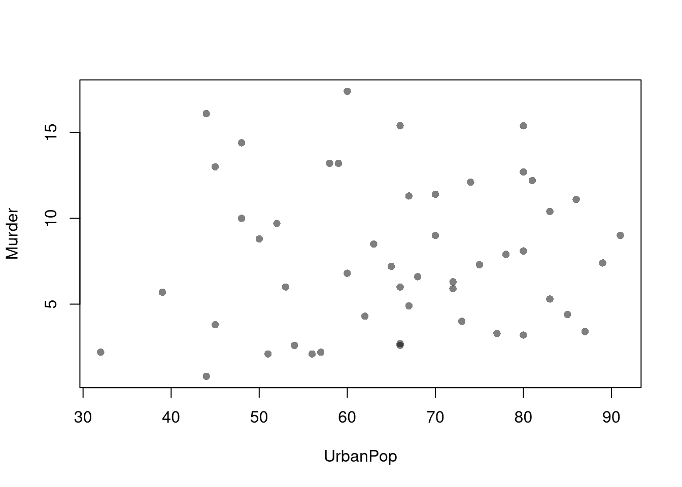
You can also show the marginal distributions of each variable along each axis.
# Setup Plot
layout( matrix(c(2,0,1,3), ncol=2, byrow=TRUE),
    widths=c(9/10,1/10), heights=c(1/10,9/10))

# Scatterplot
par(mar=c(4,4,1,1))
plot(Murder~UrbanPop, USArrests, pch=16, col=rgb(0,0,0,.5))

# Add Marginals
par(mar=c(0,4,1,1))
xhist <- hist(USArrests[,'UrbanPop'], plot=FALSE)
barplot(xhist[['counts']], axes=FALSE, space=0, border=NA)

par(mar=c(4,0,1,1))
yhist <- hist(USArrests[,'Murder'], plot=FALSE)
barplot(yhist[['counts']], axes=FALSE, space=0, horiz=TRUE, border=NA)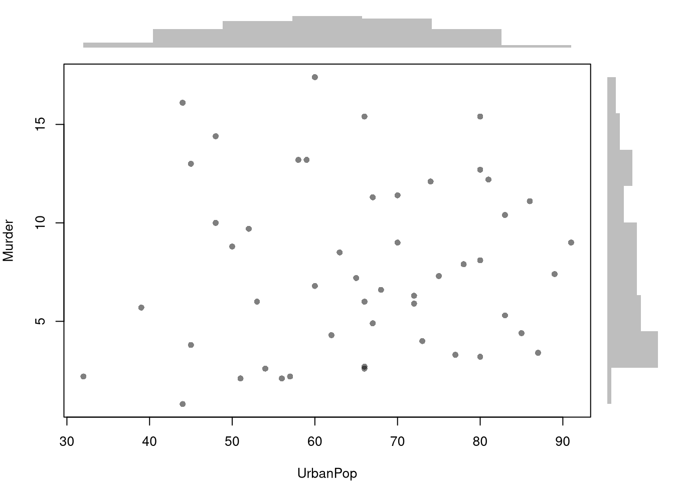
All of the univariate statistics we have covered apply to marginal distributions. For joint distributions, there are several ways to statistically describe the relationship between two variables. The major differences surround whether the data are cardinal or an ordered/unordered factor.
Pearson (Linear) Correlation. Suppose you have two vectors, \(\hat{X}\) and \(\hat{Y}\), that are both cardinal data. As such, you can compute the most famous measure of association, the covariance. Letting \(\hat{M}_{X}\) and \(\hat{M}_{Y}\) denote the mean of \(\hat{X}\) and \(\hat{Y}\), we have \[\begin{eqnarray} \hat{C}_{XY} = \sum_{i=1}^{n} [\hat{X}_{i} - \hat{M}_{X}] [\hat{Y}_i - \hat{M}_{Y}] / n \end{eqnarray}\]
Note that covariance of \(\hat{X}\) and \(\hat{X}\) is just the variance of \(\hat{X}\); \(\hat{C}_{XX}=\hat{V}_{X}\), and recall that the standard deviation is \(\hat{S}_{X}=\sqrt{\hat{V}_X}\). For ease of interpretation and comparison, we rescale the correlation statistic to always lay on a scale \(-1\) and \(+1\). A value close to \(-1\) suggests negative association, a value close to \(0\) suggests no association, and a value close to \(+1\) suggests positive association. \[\begin{eqnarray} \hat{R}_{XY} = \frac{ \hat{C}_{XY} }{ \hat{S}_{X} \hat{S}_{Y}} \end{eqnarray}\]
You can conduct hypothesis tests for these statistics using the same procedures we learned for univariate data. For example, by inverting a confidence interval.
# Load the Data
xy <- USArrests[,c('Murder','UrbanPop')]
xy_cor <- cor(xy[, 1], xy[, 2])
#plot(xy, pch=16, col=grey(0,.25))

# Bootstrap Distribution of Correlation
n <- nrow(xy)
bootstrap_cor <- vector(length=9999)
for(b in seq(bootstrap_cor) ){
    xy_b <- xy[sample(n, replace=T),]
    xy_cor_b <- cor(xy_b[, 1], xy_b[, 2])
    bootstrap_cor[b] <- xy_cor_b
}
hist(bootstrap_cor, breaks=100,
    border=NA, font.main=1,
    xlab='Correlation',
    main='Bootstrap Distribution')

## Test whether correlation is statistically different from 0
boot_ci <- quantile(bootstrap_cor, probs=c(0.025, 0.975))
abline(v=boot_ci)
abline(v=0, col='red')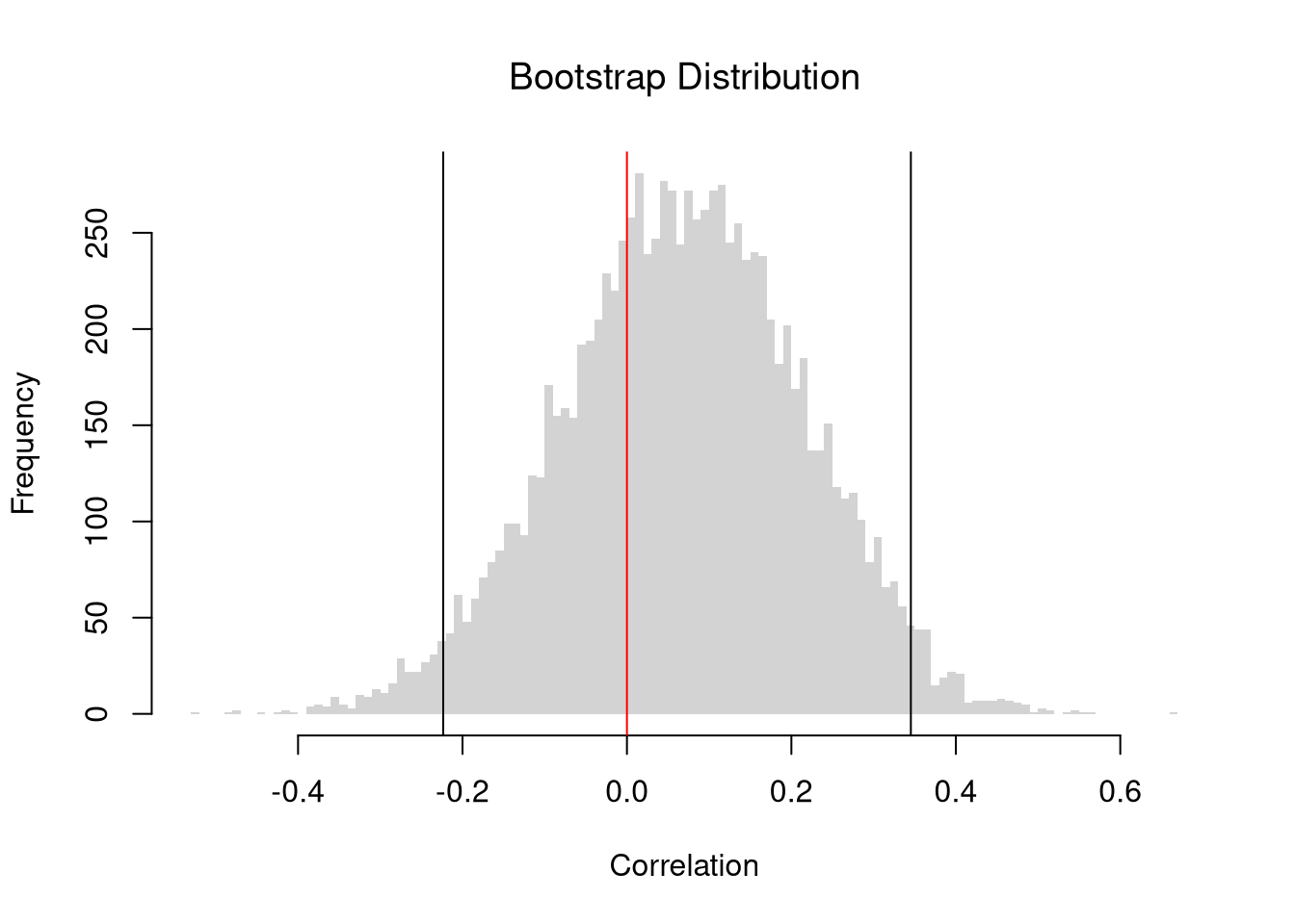
Importantly, we can also impose the null of hypothesis of no association by reshuffling the data. If we resample without replacement, this is known as a permutation test.
xy <- USArrests[,c('Murder','UrbanPop')]
xy_cor <- cor(xy[, 1], xy[, 2])
#plot(xy, pch=16, col=grey(0,.25))

# Null Bootstrap Distribution of Correlation
n <- nrow(xy)
null_bootstrap_cor <- vector(length=9999)
for(b in seq(null_bootstrap_cor) ){
    xy_b <- xy
    xy_b[,'UrbanPop'] <- xy[sample(n, replace=T),'UrbanPop'] ## Reshuffle X
    xy_cor_b <- cor(xy_b[, 1], xy_b[, 2])
    null_bootstrap_cor[b] <- xy_cor_b
}
hist(null_bootstrap_cor, breaks=100,
    border=NA, font.main=1,
    xlab='Correlation',
    main='Null Bootstrap Distribution')

## Test whether correlation is statistically different from 0
boot_ci <- quantile(null_bootstrap_cor, probs=c(0.025, 0.975))
abline(v=boot_ci)
abline(v=xy_cor, col='blue')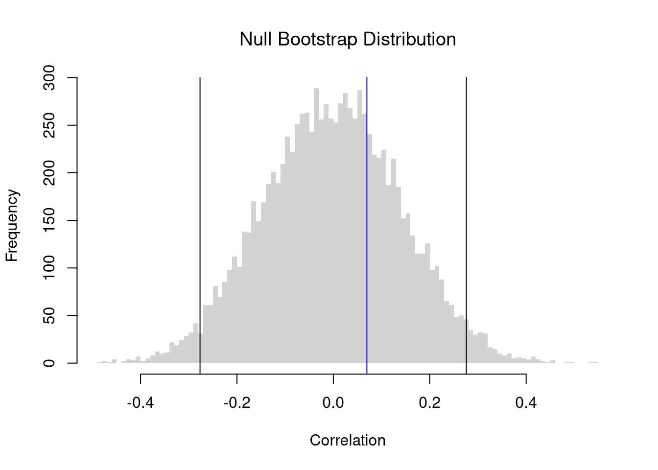
Because all dependence resides in the pairing, and permuting one margin destroys the pairing completely.
To construct a permutation test, we need to use replace=F. Rework the above code to make a Permutation Null Distribution and conduct a permutation test.
So the bootstrap evaluates sampling variability in the world that generated your data. A permutation test constructs the distribution of the statistic in a world where the null is true. Altogether, we have
| Distribution | Sample Size per Iteration | Number of Iterations | Mechanism | Typical Purpose |
|---|---|---|---|---|
| Jackknife | \(n-1\) | \(n\) | \(X,Y\): Deterministically leave-one-out observation | Variance estimate |
| Bootstrap | \(n\) | \(B\) | \(X,Y\): Random resample with replacement | Variance and CI estimate |
| Null Bootstrap | \(n\) | \(B\) | \(X,Y\): Random resample with replacement and shifted | CI under imposed null, \(p\)-values |
| Permutation | \(n\) | \(B\) | \(X\): Random resample without replacement | CI under imposed null of no association, \(p\)-values |
Falk Codeviance. The Codeviance, \(\tilde{C}_{XY}\), is a robust alternative to Covariance. Instead of relying on means (which can be sensitive to outliers), it uses medians.1 We can also scale the Codeviance by the median absolute deviation to compute the median correlation, \(\tilde{R}_{XY}\), which typically lies in \([-1,1]\) but not always. Letting \(\tilde{M}_{X}\) and \(\tilde{M}_{Y}\) denote the median of \(\hat{X}\) and \(\hat{Y}\), we have \[\begin{eqnarray} \tilde{C}_{XY} = \text{Med}\left\{ |\hat{X}_{i} - \tilde{M}_{X}| |\hat{Y}_i - \tilde{M}_{Y}| \right\} \\ \tilde{R}_{XY} = \frac{ \tilde{C}_{XY} }{ \hat{\text{MAD}}_{X} \hat{\text{MAD}}_{Y}}. \end{eqnarray}\]
codev <- function(xy) {
  # Compute medians for each column
  med <- apply(xy, 2, median)
  # Subtract the medians from each column
  xm <- sweep(xy, 2, med, "-")
  # Compute CoDev
  CoDev <- median(xm[, 1] * xm[, 2])
  # Compute the medians of absolute deviation
  MadProd <- prod( apply(abs(xm), 2, median) )
  # Return the robust correlation measure
  return( CoDev / MadProd)
}
xy_codev <- codev(xy)
xy_codev
## [1] 0.005707763
You construct sampling distributions and conduct hypothesis tests for Falk’s Codeviance statistic in the same way you do for Pearson’s Correlation statistic.
xy <- USArrests[,c('Murder','UrbanPop')]
xy_cor <- cor(xy[, 1], xy[, 2])
#plot(xy, pch=16, col=grey(0,.25))

# Null Permutation Distribution of Codeviance
n <- nrow(xy)
null_permutation_codev <- vector(length=9999)
for(b in seq(null_permutation_codev) ){
    xy_b <- xy
    xy_b[,'UrbanPop'] <- xy[sample(n, replace=F),'UrbanPop'] ## Reshuffle X
    xy_codev_b <- codev(xy_b)
    null_permutation_codev[b] <- xy_codev_b
}
hist(null_permutation_codev, breaks=100,
    border=NA, font.main=1,
    xlab='Codeviance',
    main='Null Permutation Distribution')

## Test whether correlation is statistically different from 0
abline(v=quantile(null_permutation_codev, probs=c(0.025, 0.975)))
abline(v=xy_codev, col='blue')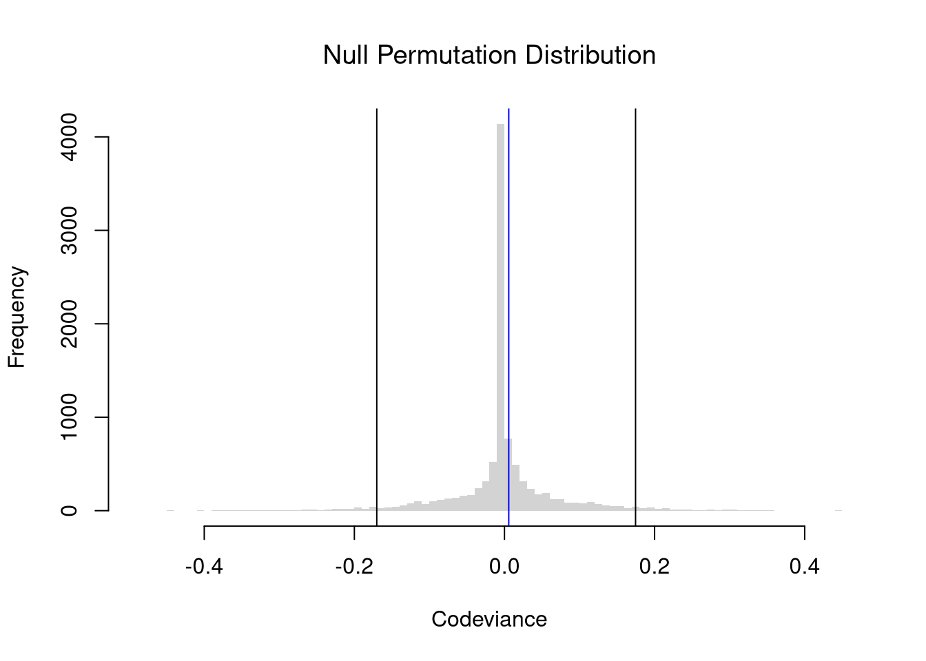
Suppose now that \(\hat{X}\) and \(\hat{Y}\) are both ordered variables. Kendall’s rank correlation statistic measures the strength and direction of association by counting the number of concordant pairs (where the ranks agree) versus discordant pairs (where the ranks disagree). A value closer to \(1\) suggests positive association in rankings, a value closer to \(-1\) suggests a negative association, and a value of \(0\) suggests no association in the ordering. \[\begin{eqnarray} \hat{KT} = \frac{2}{n(n-1)} \sum_{i} \sum_{j > i} \text{sgn} \Bigl( (\hat{X}_{i} - \hat{X}_{j})(\hat{Y}_i - \hat{Y}_j) \Bigr), \end{eqnarray}\] where the sign function is: \[\begin{eqnarray} \text{sgn}(z) = \begin{cases} +1 & \text{if } z > 0\\ 0 & \text{if } z = 0 \\ -1 & \text{if } z < 0 \end{cases}. \end{eqnarray}\]
xy <- USArrests[,c('Murder','UrbanPop')]
xy[,1] <- rank(xy[,1] )
xy[,2] <- rank(xy[,2] )
# plot(xy, pch=16, col=grey(0,.25))
KT <- cor(xy[, 1], xy[, 2], method = "kendall")
round(KT, 3)
## [1] 0.074
You construct sampling distributions and conduct hypothesis tests for Kendall’s rank correlation statistic in the same way you do as for Pearson’s Correlation statistic and Falk’s Codeviance statistic.
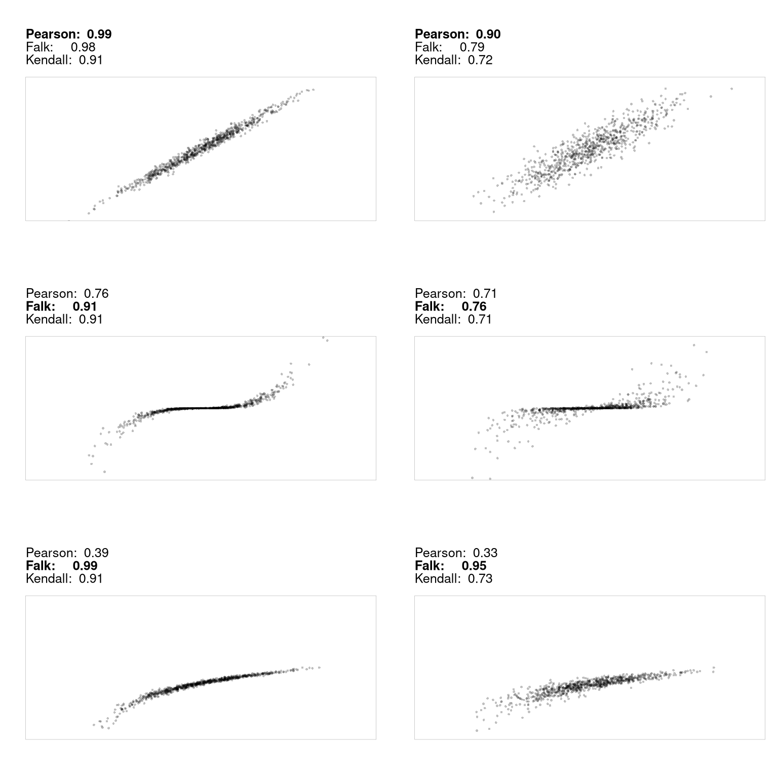
Kendall’s rank correlation coefficient can also be used for non-linear relationships, where Pearson’s correlation coefficient often falls short. It almost always helps to visual your data first before summarizing it with a statistic.
Suppose \(\hat{X}\) and \(\hat{Y}\) are both categorical variables; the value of \(\hat{X}\) is one of \(1...K\) categories and the value of \(\hat{Y}\) is one of \(1...J\) categories. We organize such data as a contingency table with \(K\) rows and \(J\) columns and use Cramer’s V to quantify the strength of association by adjusting a chi-squared statistic to provide a measure that ranges from \(0\) to \(1\); \(0\) suggests no association while a value closer to \(1\) suggests a strong association.
First, compute the chi-square statistic: \[\begin{eqnarray} \hat{\chi}^2 = \sum_{k=1}^{K} \sum_{j=1}^{J} \frac{(\hat{O}_{kj} - \hat{E}_{kj})^2}{\hat{E}_{kj}}. \end{eqnarray}\]
where
Second, normalize the chi-square statistic with the sample size and the degrees of freedom to compute Cramer’s V. Recalling that \(I\) is the number of categories for \(\hat{X}\), and \(J\) is the number of categories for \(\hat{Y}\), the statistic is \[\begin{eqnarray} \hat{CV} = \sqrt{\frac{\hat{\chi}^2 / n}{\min(J - 1, \, K - 1)}}. \end{eqnarray}\]
xy <- USArrests[,c('Murder','UrbanPop')]
xy[,1] <- cut(xy[,1],3)
xy[,2] <- cut(xy[,2],4)
table(xy)
##               UrbanPop
## Murder         (31.9,46.8] (46.8,61.5] (61.5,76.2] (76.2,91.1]
##   (0.783,6.33]           4           5           8           5
##   (6.33,11.9]            0           4           7           6
##   (11.9,17.4]            2           4           2           3

CV <- function(xy){
    # Create a contingency table from the categorical variables
    tbl <- table(xy)
    # Compute the chi-square statistic (without Yates' continuity correction)
    chi2 <- chisq.test(tbl, correct=FALSE)[['statistic']]
    # Total sample size
    n <- sum(tbl)
    # Compute the minimum degrees of freedom (min(rows-1, columns-1))
    df_min <- min(nrow(tbl) - 1, ncol(tbl) - 1)
    # Calculate Cramer's V
    V <- sqrt((chi2 / n) / df_min)
    return(V)
}
CV(xy)
## X-squared
## 0.2307071

# DescTools::CramerV( table(xy) )
You construct sampling distributions and conduct hypothesis tests for Cramer’s V statistic in the same way you do as the other statistics.
In all of the above statistics, we measure association not causation.
One major issue is statistical significance: sometimes there are relationships in the population that do not show up in samples, or non-relationships that appear in samples. This should be familiar at this point.
Other major issues pertain to real relationships averaging out and mechanically inducing relationships with random data. To be concrete about these issue, I will focus on the most-used correlation statistic and examine
Note that these are not the only examples of causation without correlation and correlation without causation. Many real datasets have temporal and spatial interdependence that create additional issues. Many real datasets also have economic interdependence, which also creates additional issues. We will delay covering these issues until much later.
Examples of this first issue includes nonlinear effects and heterogeneous effects averaging out.
set.seed(123)
n <- 10000

# X causes Y via Y = X^2 + noise
X <- runif(n, min = -1, max = 1)
epsilon <- rnorm(n, mean = 0, sd = 0.1)
Y <- X^2 + epsilon  # clear causal effect of X on Y
plot(X,Y, pch=16, col=grey(0,.1))

# Correlation over the entire range
title( paste0('Cor: ', round( cor(X, Y), 1) ) ,
    font.main=1)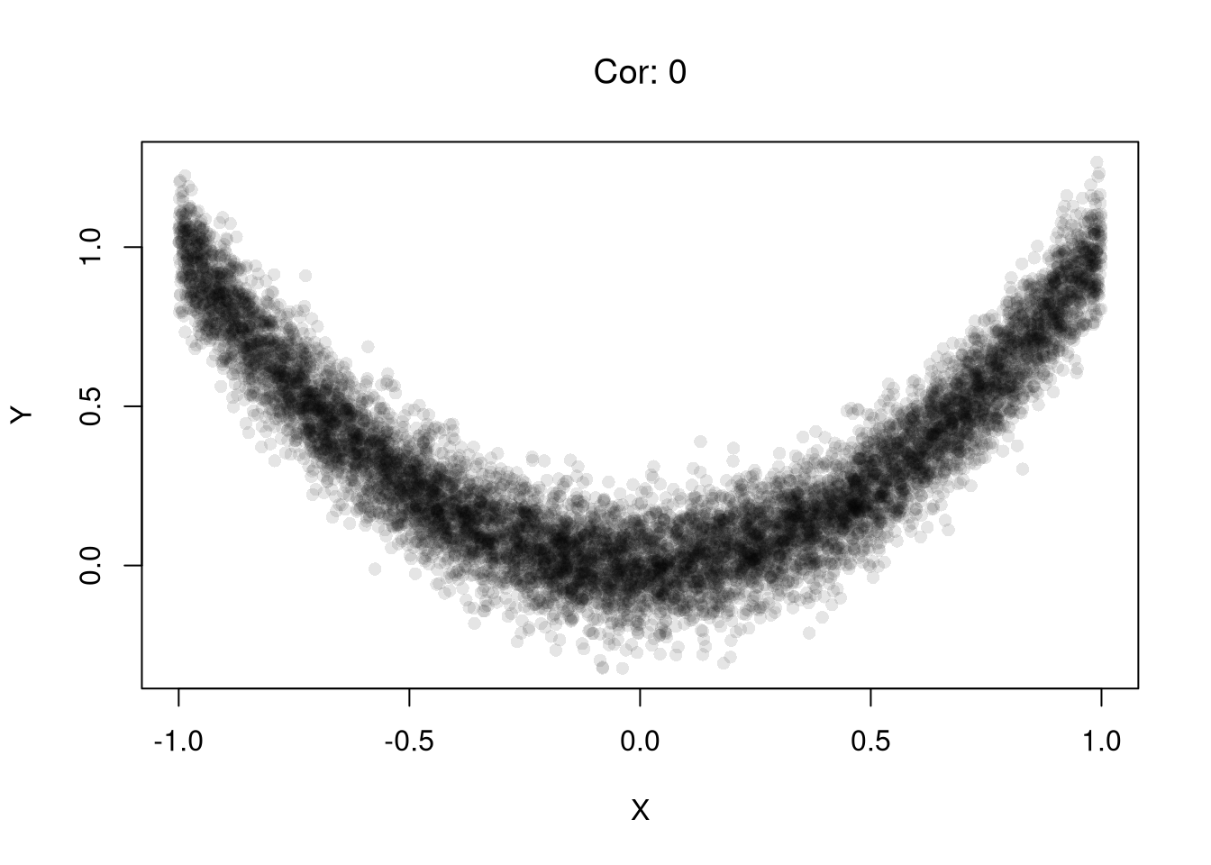
# Heterogeneous Effects
X <- rnorm(n) # Randomized "treatment"

# Heterogeneous effects based on group
group <- rbinom(n, size = 1, prob = 0.5)
epsilon <- rnorm(n, mean = 0, sd = 1)
Y <- ifelse(group == 1,
            X + epsilon,   # positive effect
            -X + epsilon)  # negative effect
plot(X,Y, pch=16, col=grey(0,.1))

# Correlation in the pooled sample
title( paste0('Cor: ', round( cor(X, Y), 1) ),
    font.main=1 )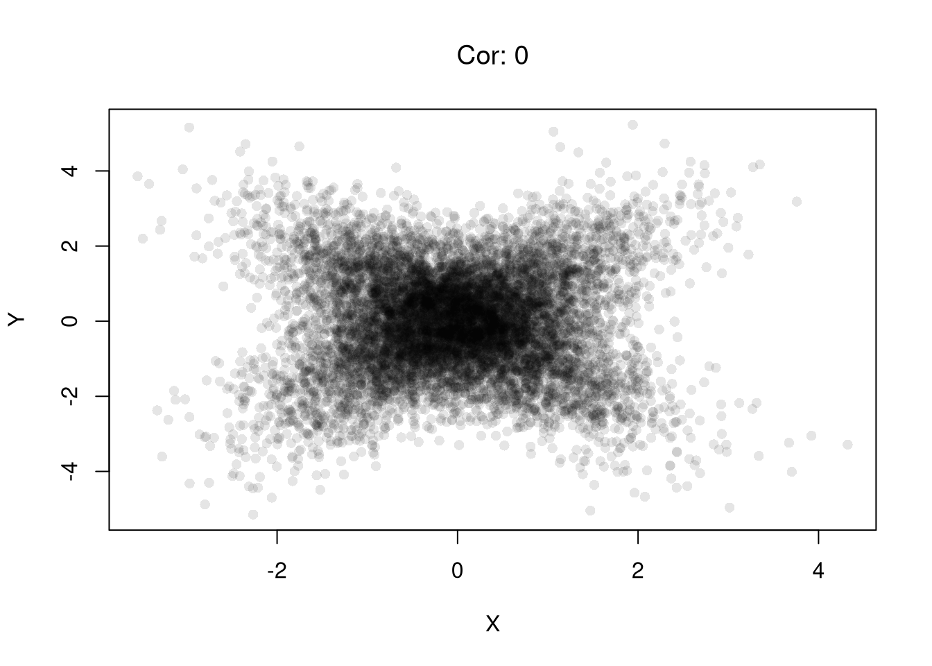
Examples of this second issue includes shared denominators and selection bias inducing correlations.
Consider three completely random variables. We can induce a mechanical relationship between the first two variables by dividing them both by the third variable.
set.seed(123)
n <- 20000

# Independent components
A <- runif(n)
B <- runif(n)
C <- runif(n)
par(mfrow=c(1,2))
plot(A,B, pch=16, col=grey(0,.1))
title('Independent Variables', font.main=1)

# Ratios with a shared denominator
X <- A / C
Y <- B / C
plot(X,Y, pch=16, col=grey(0,.1))
title('With Common Divisor', font.main=1)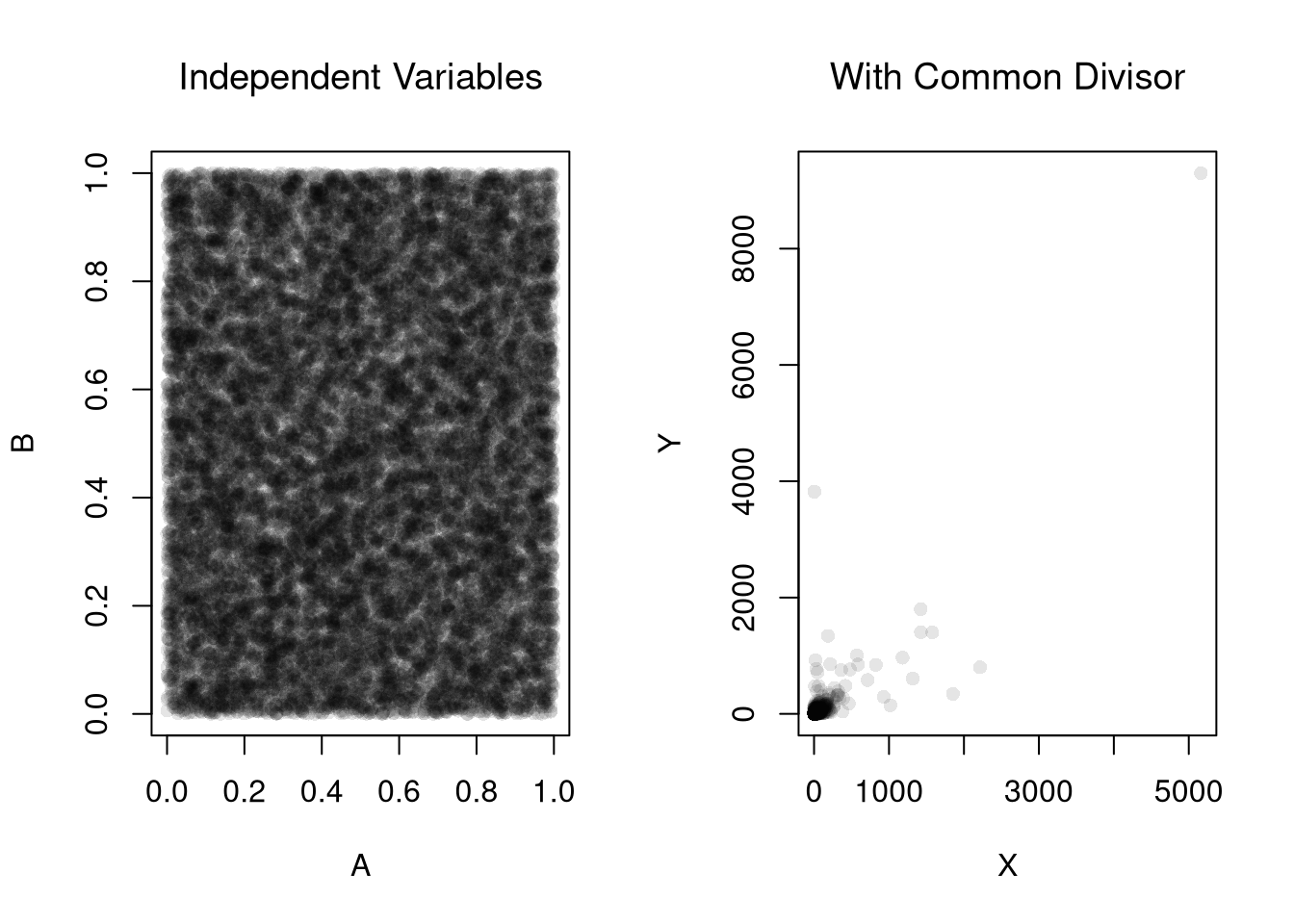
# Correlation
cor(X, Y)
## [1] 0.8183118
Consider an admissions rule into university: applicants are accepted if they have either high test scores or strong extracurriculars. Even if there is no general relationship between test scores and extracurriculars, you will see one amongst university students.
# Independent traits in the population
test_score        <- rnorm(n, mean = 0, sd = 1)
extracurriculars  <- rnorm(n, mean = 0, sd = 1)

# Selection above thresholds
threshold <- 1.0
admitted <- (test_score > threshold) | (extracurriculars > threshold)
mean(admitted)  # admission rate
## [1] 0.29615

par(mfrow = c(1, 2))
# Full population
plot(test_score, extracurriculars,
     pch=16, col=grey(0,.1))
title('General Sample', font.main=1)
# Admitted only
plot(test_score[admitted], extracurriculars[admitted],
     pch=16, col=grey(0,.1))
title('University Sample', font.main=1)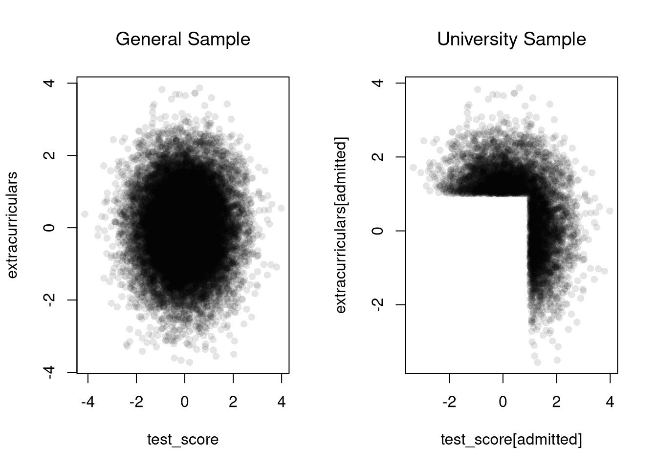
# Correlation among admitted applicants only
cor(test_score[admitted], extracurriculars[admitted])
## [1] -0.5597409For plotting histograms and marginal distributions, see
Other Statistics
See also Theil-Sen Estimator, which may be seen as a precursor.↩︎