We will now dig a little deeper theoretically into the statistics we compute. When we know how the data are generated theoretically, we can often compute the theoretical value of the two most basic and often-used statistics: the mean and variance. Recall that we denote \(X_{i}\) as a random variable that can take on specific values \(x\) from the sample space with known probabilities (see this probability refresher if needed). For example, \(X_{i}\) is a coin that we will flip and it can land on heads (\(x=1\)) or tails (\(x=0\)).
\(X_{i}\) is a random variable, taking on outcomes \(x\)
\(\hat{X}_{i}\) is a realized value
The theoretical mean, \(\mu\), and variance, \(\sigma^2\), describe the population distribution \(F\) generating the data. The population parameters (\(\mu, \sigma^2\)) are fixed, true values. They are often unknown and estimated with sample statistics that are calculated from data. With sample statistics, you should distinguish the particular estimate you calculated for your sample, \(\hat{M}\), and the estimator\(M\) that is computed on any sample. For example, consider flipping a coin three times: \(M\) corresponds to a theoretical formula you compute on coins before they are flipped and \(\hat{M}\) corresponds to a specific value after you flip the coins.
Statistical definitions
Concept
Mean
Variance
What it is
Terminology
Alternative Terminology
Estimate
\(\hat{M}\)
\(\hat{V}\)
one number you compute for a single sample of size \(n\)
a random variable, formula that computes the statistic for any sample of size \(n\)
Population
\(\mu\)
\(\sigma^2\)
a number defined by the theoretical distribution
theoretical mean, variance
population/long-run mean, variance
For concreteness, we separately analyze how the theoretical mean and variance are computed for discrete and continuous random variables.
6.1 Population Parameters
Discrete Random Variables.
If the sample space is discrete, we can compute the expected value, or theoretical mean, as \[\begin{eqnarray}
\mu = \mathbb{E}[X_{i}] = \sum_{x} x Prob(X_{i}=x),
\end{eqnarray}\] where \(\mathbb{E}\) is the expectation function that explicitly uses the population distribution via \(Prob(X_{i}=x)\): the probability the random variable \(X_{i}\) takes the particular value \(x\). Similarly, we can compute the population variance as \[\begin{eqnarray}
\sigma^2 = \mathbb{V}[X_{i}] = \mathbb{E}[(X_{i}-\mu)^2] = \sum_{x} \left(x - \mu \right)^2 Prob(X_{i}=x),
\end{eqnarray}\] where \(\mathbb{V}\) is the variance function which also explicitly uses the population distribution. The population standard deviation is \(\sigma = \sqrt{\mathbb{V}[X_{i}]}\), which measures the spread of the distribution of individual outcomes around the theoretical mean.
For example, consider a five-sided die with equal probability of landing on each side. I.e., \(X_{i}\) is a Discrete Uniform random variable with outcomes \(x \in \{1,2,3,4,5\}\). What is the theoretical mean? What is the variance and standard deviation? \[\begin{eqnarray}
\mu &=& \mathbb{E}[X_{i}] = 1\frac{1}{5} + 2\frac{1}{5} + 3\frac{1}{5} + 4\frac{1}{5} + 5\frac{1}{5} = 15/5 = 3\\
\sigma^2 = \mathbb{V}[X_{i}] &=& (1-3)^2\frac{1}{5} +
(2 - 3)^2\frac{1}{5} +
(3 - 3)^2\frac{1}{5} +
(4 - 3)^2\frac{1}{5} +
(5 - 3)^2\frac{1}{5} \\
&=& 2^2 \frac{1}{5} + 1^2\frac{1}{5} + 0^2 \frac{1}{5} + 1^2\frac{1}{5} + 2^2 \frac{1}{5}
= (4 + 1 + 1 + 4)/5 = 10/5 = 2\\
\sigma &=& \sqrt{2}
\end{eqnarray}\]
Code
# Computerized Way to Compute Meanx <-c(1, 2, 3, 4, 5)x_probs <-c(1/5, 1/5, 1/5, 1/5, 1/5)X_mean <-sum(x*x_probs)X_mean## [1] 3# Computerized Way to Compute SDXvar <-sum((x-X_mean)^2*x_probs)Xvar## [1] 2Xsd <-sqrt(Xvar)Xsd## [1] 1.414214# Verified by simulationXsim <-sample(x, prob=x_probs,size=10000, replace=T)mean(Xsim)## [1] 2.9909sd(Xsim)## [1] 1.39879
NoteMust Know
For example, consider an unfair coin with a \(3/4\) probability of heads (\(x=1\)) and a \(1/4\) probability of tails (\(x=0\)) has a theoretical mean of \[\begin{eqnarray}
\mathbb{E}[X_{i}] = 0\frac{1}{4} + 1\frac{3}{4} = \frac{3}{4}
\end{eqnarray}\] and a theoretical variance of \[\begin{eqnarray}
\mathbb{V}[X_{i}] = [0 - \frac{3}{4}]^2 \frac{1}{4} + [1 - \frac{3}{4}]^2 \frac{3}{4}
= \frac{9}{64} + \frac{3}{64}
= \frac{12}{64}
= \frac{3}{16}.
\end{eqnarray}\] Verify both the mean and variance by simulation.
Code
# A simulation of many coin flipsx <-c(0, 1)x_probs <-c(1/4, 3/4)X <-sample(x, prob=x_probs, size=1000, replace=T)round( mean(X), 4)## [1] 0.732round( var(X), 4)## [1] 0.1964
NoteMust Know
Consider a four-sided die with outcomes \(\{1,2,3,4 \}\) and corresponding probabilities \(\{ 1/8, 2/8, 1/8, 4/8 \}\) . What is the mean? \[\begin{eqnarray}
\mathbb{E}[X_{i}] = 1 \frac{1}{8} + 2 \frac{2}{8} + 3 \frac{1}{8} + 4 \frac{4}{8} = 3
\end{eqnarray}\] What is the variance? Verify both the mean and variance by simulation.
TipTest Yourself
Consider an unfair coin with a \(p\) probability of heads (\(x=1\)) and a \(1-p\) probability of tails (\(x=0\)), where \(p\) is a parameter between \(0\) and \(1\). The theoretical mean is \[\begin{eqnarray}
\mathbb{E}[X_{i}] = 1[p] + 0[1-p] = p
\end{eqnarray}\] and the theoretical variance is \[\begin{eqnarray}
\mathbb{V}[X_{i}]
= [1 - p]^2 p + [0 - p]^2 [1-p] = [1 - p]^2 p + p^2 [1-p]
= [1-p]p\left( [1-p] + p\right) = [1-p] p.
\end{eqnarray}\] So the theoretical standard deviation is \(\sigma=\sqrt{[1-p] p}\).
TipTest Yourself
Suppose \(X_{i}\) is a discrete random variable with this probability mass function: \[\begin{eqnarray}
X_{i} &=& \begin{cases}
-1 & \text{ with probability } \frac{1}{2 \lambda^2} \\
0 & \text{ with probability } 1-\frac{1}{\lambda^2} \\
+1 & \text{ with probability } \frac{1}{2\lambda^2}
\end{cases},
\end{eqnarray}\] where \(\lambda>0\) is a parameter. What is the theoretical standard deviation?
TipTest Yourself
For a discrete uniform random variable with the sample space \(\{1,2,3,4,5\}\), calculate the theoretical median and IQR.
Law of the Unconscious Statistician (LOTUS).
As before, we will represent the random variable as \(X_{i}\), which can take on values \(x\) from the sample space. If \(X_{i}\) is a discrete random variable (a random variable with a discrete sample space) and \(g\) is a function, then \(\mathbb E[g(X_{i})] = \sum_x g(x)Prob(X_{i}=x)\).
TipTest Yourself
Let \(X_{i}\) take values \(\{1,2,3\}\) with \[\begin{eqnarray}
Prob(X_{i}=1)=0.2,\quad Prob(X_{i}=2)=0.5,\quad Prob(X_{i}=3)=0.3.
\end{eqnarray}\] Let \(g(x)=x^2+1\). Then \(g(1)=1^2+1=2\), \(g(2)=2^2+1=5\), \(g(3)=3^2+1=10\).
g <-function(x) x^2+1# A theoretical examplex <-c(1, 2, 3, 4)x_probs <-c(1/4, 1/4, 1/4, 1/4)sum(g(x) * x_probs) ## [1] 8.5# A simulation exampleX <-sample(x, prob=x_probs, size=1000, replace=T)mean(g(X))## [1] 8.779
TipTest Yourself
If \(X_{i}\) is a continuous random variable (a random variable with a continuous sample space) and \(g\) is a function, then \(\mathbb E[g(X_{i})] = \int_{-\infty}^{\infty} g(x)f(x) dx\).
Code
x <-rexp(5e5, rate =1) # X ~ Exp(1)mean(sqrt(x)) # LOTUS Simulation## [1] 0.8859465sqrt(pi) /2# Exact via LOTUS integral## [1] 0.8862269
Note that you have already seen the special case where \(g(X_{i})=\left(X_{i}-\mathbb{E}[X_{i}]\right)^2\). LOTUS also applies to continuous random variables.
Continuous Random Variables.
Many continuous random variables are parameterized by their means and variances. For example, the exponential distribution has a rate parameter \(\lambda\), which corresponds to the theoretical mean \(1/\lambda\) and variance \(1/\lambda^2\). For another example, the two parameters of the normal distribution are \(\mu\) and \(\sigma^2\), which corresponds to the theoretical mean and variance.
Code
# Exponential Random VariableX <-rexp(5000, 2)m <-mean(X)round(m, 2)## [1] 0.5# Normal Random VariableX <-rnorm(5000, 1, 2)round(mean(X), 2)## [1] 1.02round(var(X), 2)## [1] 4.14
Advanced and Optional
If the sample space is continuous, we can compute the theoretical mean (or expected value) as \[\begin{eqnarray}
\mathbb{E}[X] = \int x f(x) d x,
\end{eqnarray}\] where \(f(x)\) is the probability density for the particular value \(x\). Note that this is not a probability; probabilities are areas under \(f\).
Similarly, we can compute the theoretical variance as \[\begin{eqnarray}
\mathbb{V}[X_{i}]= \int \left(x - \mathbb{E}[X_{i}] \right)^2 f(x) d x,
\end{eqnarray}\]
For example, consider a random variable with a continuous uniform distribution over \([-1, 1]\). In this case, \(f(x)=1/[1 - (-1)]=1/2\) for each \(x \in [-1, 1]\) and \[\begin{eqnarray}
\mathbb{E}[X_{i}] = \int_{-1}^{1} \frac{x}{2} d x = \int_{-1}^{0} \frac{x}{2} d x + \int_{0}^{1} \frac{x}{2} d x = 0
\end{eqnarray}\] and \[\begin{eqnarray}
\mathbb{V}[X_{i}]= \int_{-1}^{1} x^2 \frac{1}{2} d x = \frac{1}{2} \frac{x^3}{3}|_{-1}^{1} = \frac{1}{6}[1 - (-1)] = 2/6 =1/3
\end{eqnarray}\]
You can estimate probabilities with data. With discrete data there are a limited number of unique outcomes, and we can estimate the probability of each outcome as \[\begin{eqnarray}
\hat{p}_{x}=\sum_{i=1}^{n}\mathbf{1}\left( \hat{X}_{i}=x\right)/n,
\end{eqnarray}\] where \(x\) is one particular value of interest. We often estimate the probabilities for each unique outcome.
NoteMust Know
Suppose there is an experiment with three possible outcomes, \(\{A, B, C\}\). It was repeated \(50\) times and discovered that \(A\) occurred \(10\) times, \(B\) occurred \(13\) times, and \(C\) occurred \(27\) times. The estimated probability of each outcome is found via the bar plot \(\hat{p}_{A} = 10/50\), \(\hat{p}_{B} = 13/50\), \(\hat{p}_{C} = 27/50\). We can also estimate the “in” probabilities as \(\hat{Prob}(A \text{ or } B)=10/50+13/50=23/50\) and \(\hat{Prob}(B \text{ or } C)=13/50+27/50=40/50\), as well as the “out” probability as \(\hat{Prob}(A \text{ or } C)=10/50+27/50=37/50\).
Do these calculations with the computer.
Sometimes, you may have a dataset of values and probability weights. In any case, we can then estimate the population mean via \[\begin{eqnarray}
\hat{M} &=& \sum_{x} x \hat{p}_{x},
\end{eqnarray}\] which is equivalent to the sample mean.
NoteMust Know
Suppose we flipped a coin \(100\) times and found that \(76\) were heads and \(24\) were tails. The estimated probabilities are \(76/100\) for the outcome \(X_{i}=1\) and \(24/100\) for the outcome \(X_{i}=0\). We compute the mean as \(\hat{M}=1\times 0.76 + 0 \times 0.24 = 0.76\).
Note that we get the same number if we instead computed \(\sum_{i} \hat{X}_{i}/100 = [\sum_{i=1}^{24} 0/100 + \sum_{i=25}^{100} 1/100 = [100-24]/100 = 0.76.\)
Code
# Simulate the coin flipsX <-sample(c(0, 1), 100, prob=c(0.24, 0.76), replace=T)# Compute a sample estimate using probability weightsP <-table(X) #table of countsp <-c(P)/length(X) #frequencies (must sum to 1)x <-as.numeric(names(p)) #unique valuescbind(x, p)## x p## 0 0 0.24## 1 1 0.76# Sample Mean EstimateX_mean <-sum(x*p)X_mean## [1] 0.76mean(X)## [1] 0.76
TipTest Yourself
Try estimating the sample mean the two different ways for another random sample
Code
x <-c(0, 1, 2)x_probs <-c(1/3, 1/3, 1/3)X <-sample(x, prob=x_probs, 1000, replace=T)# First Way (Computerized)mean(X)## [1] 0.988# Second Way (Explicit Calculations)# start with a table of counts like the previous example
The weighting idea generalizes to other statistics. E.g., we can also estimate variance with probability weights
TipTest Yourself
Provide a concrete example of computing a weighted variance building on this code below
You can estimate means and variances for continuous random variables with weights, but here we have an additional approximation error due to binning by the histogram.
Code
# values and probabilitiesh <-hist(X, plot=F)wt <- h[['counts']]/length(X) xt <- h[['mids']]# Weighted meanX_mean <-sum(wt*xt)X_mean## [1] 0.9572# Compare to 'mean(x)'
Try it yourself with
Code
X <-runif(2000, -1, 1)
6.3 Estimators
Means.
The LLN relates to a famous theoretical result in statistics, Linearity of Expectations: the expected value of a sum of random variables equals the sum of their individual expected values (see here for a detailed treatment). To be concrete, suppose we take \(n\) random variables, each one denoted as \(X_{i}\). Then, for constants \(a,b,1/n\), we have \[\begin{eqnarray}
\mathbb{E}[a X_{1}+ b X_{2}] &=& a \mathbb{E}[X_{1}]+ b \mathbb{E}[X_{2}]\\
\mathbb{E}\left[M\right] &=& \mathbb{E}\left[ \sum_{i=1}^{n} X_{i}/n \right] = \sum_{i=1}^{n} \mathbb{E}[X_{i}]/n
\end{eqnarray}\] Assuming each data point has an identical mean; \(\mathbb{E}[X_{i}]=\mu\), the expected value of the sample average is the mean; \(\mathbb{E}\left[M\right] = \sum_{i=1}^{n} \mu/n = \mu\).
TipTest Yourself
For example, consider a coin flip with Heads \(X_{i}=1\) having probability \(p\) and Tails \(X_{i}=0\) having probability \(1-p\). First notice that \(\mathbb{E}[X_{i}]=p\). Then notice we can first \[\begin{align*}
\mathbb{E}[X_{1}+X_{2}]
&= [1+1][p \times p] + [1+0][p \times (1-p)] + [0+1][(1-p) \times p] + [0+0][(1-p) \times (1-p)] & \text{``HH + HT + TH + TT''} \\
&= [1][p \times p] + [1][p \times (1-p)] + [0][(1-p) \times p] + [0][(1-p) \times (1-p)] & \text{first outcomes times prob.} \\
&+ [1][p \times p] + [0][p \times (1-p)] + [1][(1-p) \times p] + [0][(1-p) \times (1-p)] &
\text{+second outcomes times prob.} \\
&= [1][p \times p] + [1][p \times (1-p)] + [1][p \times p] + [1][(1-p) \times p] & \text{drop zeros}\\
&= 1p (p + [1-p]) + 1p (p + [1-p]) = p+p & \text{algebra}\\
&= \mathbb{E}[X_{1}] + \mathbb{E}[X_{2}] .
\end{align*}\] The theoretical mean is \(\mathbb{E}[\frac{X_{1}+X_{2}}{2}]=\frac{p+p}{2}=p\).
Variances.
Another famous theoretical result in statistics is that if we have independent and identical data (i.e., that each random variable \(X_{i}\) has the same mean \(\mu\), same variance \(\sigma^2\), and is drawn without any dependence on the previous draws), then the standard error of the sample mean decreases by \(1/\sqrt{n}\). Intuitively, this follows from thinking of the variance as a type of mean (the mean squared deviation from \(\mu\)). \[\begin{eqnarray}
\mathbb{V}\left[ M \right]
&=& \mathbb{V}\left[ \frac{\sum_{i=1}^{n} X_{i}}{n} \right]
= \sum_{i=1}^{n} \mathbb{V}\left[\frac{X_{i}}{n}\right]
= \sum_{i=1}^{n} \frac{\sigma^2}{n^2}
= \sigma^2/n\\
SE\left(M\right) &=& \sqrt{\mathbb{V}\left[ M \right] } = \sqrt{\sigma^2/n} = \sigma/\sqrt{n}.
\end{eqnarray}\]
Note that the standard deviation refers variability of individual observations (in either a sample or population), and is hence different from the standard error. To be clear,
Types of variability
Concept
What varies
Notation
Standard deviation
individual observations within a sample or population
\(\hat{S}\) or \(\sigma\)
Standard error
a statistic across samples
\(SE(M)\)
Nonetheless, the sample standard deviation can be used to estimate the standard error of the sample mean. Specifically, assume that the data are approximately i.i.d and approximate the population standard deviation, \(\sigma\), with the sample standard deviation, \(\hat{S}\); \[\begin{eqnarray}
SE(M) \approx \sigma/\sqrt{n} \approx \hat{S}/\sqrt{n}.
\end{eqnarray}\]
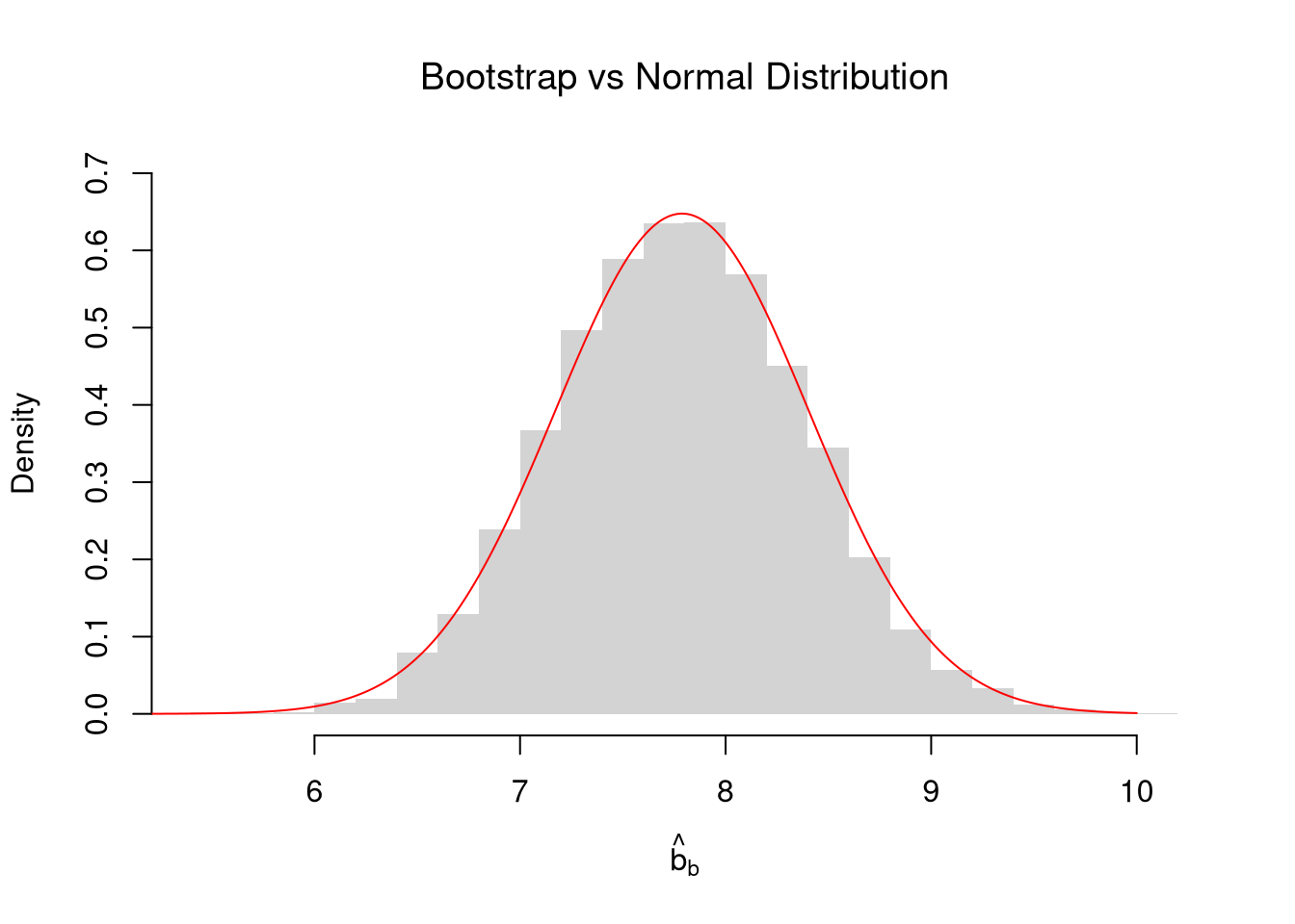
Another data-driven way is to create a bootstrap distribution for the sample mean and then compute the standard deviation of the bootstrap distribution \(\hat{SE}^{\text{boot}} \approx SE(M)\). The theory-driven estimate is often a little different from the bootstrap estimate, as the theory-driven estimate is based on idealistic assumptions (i.i.d. and normality) whereas the bootstrap estimate is driven by data that are often not ideal. The theory-driven estimate does have some advantages too, but we do not go into that as we would need more advanced mathematics.
Sometimes, the sampling distribution is approximately normal due to the CLT. With the sample mean \(M\) being approximately normal alongside i.i.d data, the distribution of \(M\) is approximately \(Normal(\mu, \hat{S}/\sqrt{n})\).
Code
# Bootstrap Distributionhist(bootstrap_means, breaks=25,main=NA, border=NA,freq=F, ylim=c(0, 0.7),xlab=expression(hat(b)[b]))title('Bootstrap vs Normal Distribution', font.main=1)# Theoretical Distribution: Normal Approximation with IID SEsx <-seq(5, 10, by=0.01)fx <-dnorm(x, mean(sample_dat), theory_se)lines(x, fx, col=rgb(1, 0, 0, .8), lty=1)
6.4 Exercises
Explain in your own words the difference between an estimate \(\hat{M}\), an estimator \(M\), and a population parameter \(\mu\). Why is it important to distinguish between these three concepts?
Suppose \(X_{i}\) is a discrete random variable with outcomes \(\{1, 3, 5, 7\}\) and corresponding probabilities \(\{0.1, 0.2, 0.4, 0.3\}\). Compute the theoretical mean \(\mu\), variance \(\sigma^2\), and standard deviation \(\sigma\) by hand. Verify your answers using R.
Using the USArrests dataset in R, compute the sample mean and the bootstrap standard error of the mean for the Assault variable. Then compute the theory-driven standard error \(\hat{S}/\sqrt{n}\) and compare the two estimates.