# Simulate Bivariate Data
N <- 10000
Mu <- c(2,2) ## Means
Sigma1 <- matrix(c(2,-.8,-.8,1),2,2) ## CoVariance Matrix
MVdat1 <- mvtnorm::rmvnorm(N, Mu, Sigma1)
colnames(MVdat1) <- c('X','Y')
Sigma2 <- matrix(c(2,.4,.4,1),2,2) ## CoVariance Matrix
MVdat2 <- mvtnorm::rmvnorm(N, Mu, Sigma2)
colnames(MVdat2) <- c('X','Y')
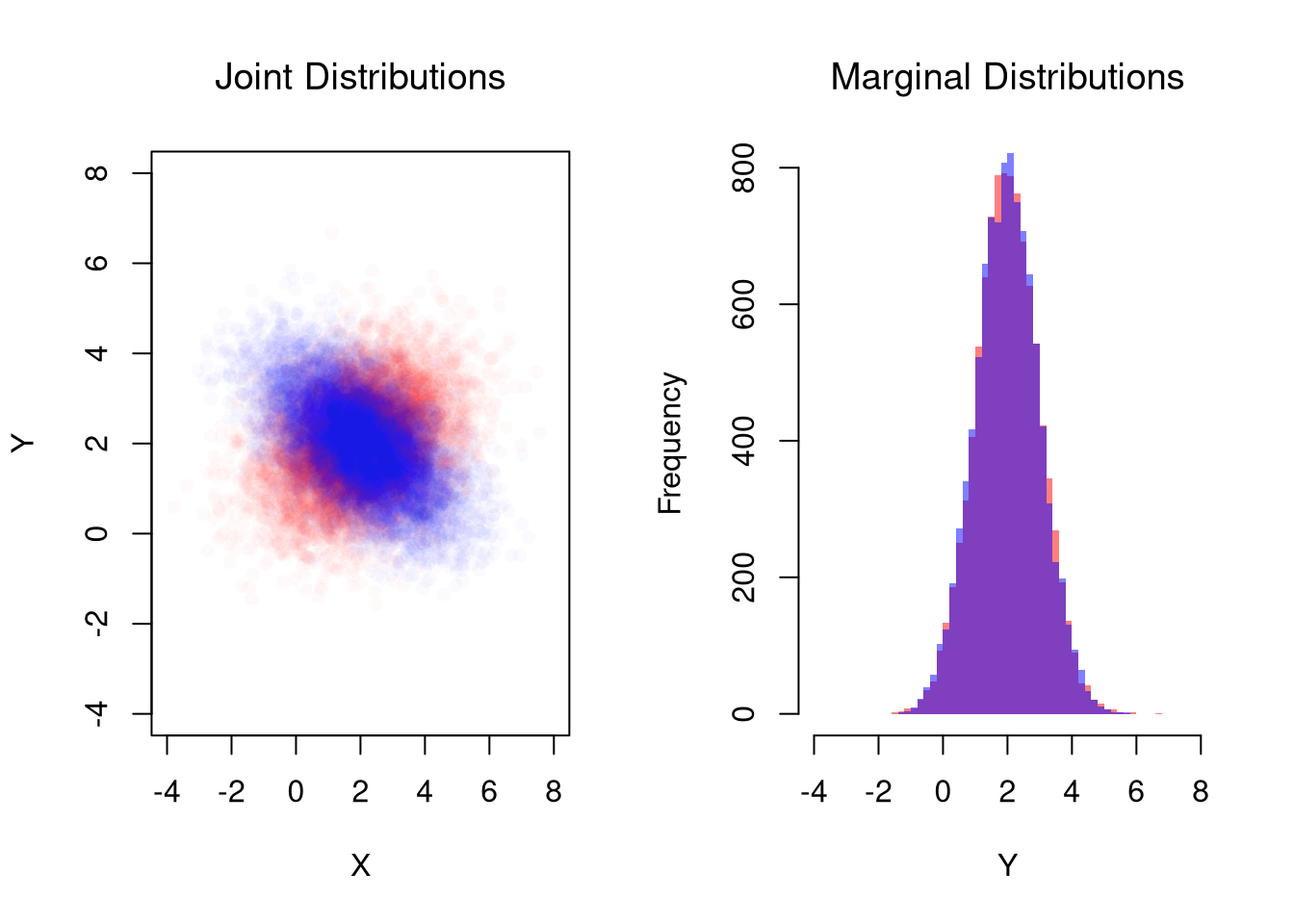
par(mfrow=c(1,2))
## Different diagonals
plot(MVdat2, col=rgb(1,0,0,0.02), pch=16,
main='Joint Distributions', font.main=1,
ylim=c(-4,8), xlim=c(-4,8),
xlab='X', ylab='Y')
points(MVdat1,col=rgb(0,0,1,0.02),pch=16)
## Same marginal distributions
xbks <- seq(-4,8,by=.2)
hist(MVdat2[,2], col=rgb(1,0,0,0.5),
breaks=xbks, border=NA,
xlab='Y',
main='Marginal Distributions', font.main=1)
hist(MVdat1[,2], col=rgb(0,0,1,0.5),
add=T, breaks=xbks, border=NA)