13  Simple Regression

---

Suppose we have some bivariate data: \(\hat{X}_{i}, \hat{Y}_{i}\). In the previous chapter, we summarized the strength of association between two variables using correlation. Correlation tells us how strongly \(X\) and \(Y\) move together, but not by how much \(Y\) changes per unit change in \(X\). Regression answers that question by fitting a line through the data.

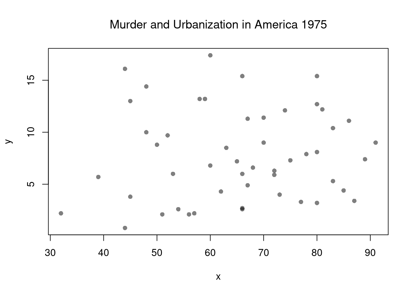
# Pull two columns from USArrests and rename for compact code below
xy <- USArrests[, c('Murder', 'UrbanPop')]
colnames(xy) <- c('y', 'x')                     # y=outcome, x=predictor

# Scatter the data
plot(y ~ x, xy, col=grey(0, .5), pch=16,
    main=NA,
    xlab='Population Share in Urban Area',
    ylab='Murder Arrests per 100K')
title('Data from American States, 1975', font.main=1)

cor(xy$x, xy$y)                                 # Pearson correlation
## [1] 0.06957262

# Slope from correlation: R_{XY} * S_Y / S_X
cor(xy$x, xy$y) * sd(xy$y)/sd(xy$x)
## [1] 0.02093466

# Fit the line via OLS and overlay it on the scatter
reg <- lm(y ~ x, data=xy)
abline(reg, lty=2)

ImportantKey Definition

A fitted value \(\hat{y}_{i}\) is the regression line evaluated at the \(i\)-th observation’s \(\hat{X}_{i}\).

The sample residual is the gap between actual and fitted, \(\hat{e}_{i} = \hat{Y}_{i} - \hat{y}_{i}\).

13.1 Simple Linear Regression

This refers to fitting a linear model to bivariate data.

Model and Objective.

A regression line goes through the cloud of points. To calculate it, we need some definitions first.

ImportantKey Definition

Our simple linear model is \[\begin{eqnarray} \hat{Y}_{i}=b_{0}+b_{1} \hat{X}_{i}+e_{i}, \end{eqnarray}\] where \(b_{0}\) and \(b_{1}\) are parameters (the coefficients), and \(\hat{X}_{i}, \hat{Y}_{i}\) are the data for observation \(i\).

The residual \(e_{i}\) is the vertical gap between observation \(i\)’s actual value of \(\hat{Y}_{i}\) and the model’s prediction for that observation: \[e_{i}=\hat{Y}_{i}-(b_{0}+b_{1}\hat{X}_{i}).\] We find the parameters which best-fit the data, by minimizing the sum of squared residuals. We used squared residuals to prevent positive and negative errors from cancelling and penalizes big misses more than small ones.

ImportantKey Definition

The ordinary least-squares (OLS) coefficients minimize the sum of squared residuals. \[\begin{eqnarray} \min_{b_{0}, b_{1}} \sum_{i=1}^{n} \left( e_{i} \right)^2 &=& \min_{b_{0}, b_{1}} \sum_{i=1}^{n} \left( \hat{Y}_{i} - [b_{0}+b_{1} \hat{X}_{i}] \right)^2. \end{eqnarray}\]

The OLS problem has a closed-form solution. The optimal OLS slope and intercept are \[\hat{b}_{1} = \frac{\hat{C}_{XY}}{\hat{V}_{X}}, \qquad \hat{b}_{0} = \hat{M}_{Y} - \hat{b}_{1} \hat{M}_{X}.\]

The least-squares slope \(\hat{b}_{1}\) is useful as the canonical “how much does fitted \(\hat{Y}\) change per one-unit change in \(\hat{X}\)” summary, and the formula shows it is just the covariance divided by the variance of \(X\). Equivalently, \(\hat{b}_{1} = \hat{R}_{XY} \cdot \hat{S}_{Y}/\hat{S}_{X}\), so the slope is the Pearson correlation rescaled by the ratio of standard deviations. The intercept formula then guarantees the fitted line passes through the point of means \((\hat{M}_{X}, \hat{M}_{Y})\).

To derive these, take partial derivatives of the objective with respect to each coefficient and set to zero. For the slope: \[\begin{eqnarray} 0 &=& \sum_{i=1}^{n} 2\left( \hat{Y}_{i} - [b_{0}+b_{1} \hat{X}_{i}] \right) \hat{X}_{i} \\ \Rightarrow \hat{b}_{1} &=& \frac{\sum_{i=1}^{n}(\hat{X}_{i}-\hat{M}_{X})(\hat{Y}_{i}-\hat{M}_{Y})}{\sum_{i=1}^{n}(\hat{X}_{i}-\hat{M}_{X})^2} = \frac{\hat{C}_{XY}}{\hat{V}_{X}}. \end{eqnarray}\] For the intercept: \[\begin{eqnarray} 0 &=& \sum_{i=1}^{n} 2\left( \hat{Y}_{i} - [b_{0}+b_{1} \hat{X}_{i}] \right)\\ \Rightarrow \hat{b}_{0} &=& \hat{M}_{Y}-\hat{b}_{1}\hat{M}_{X} . \end{eqnarray}\] We could alternatively find the best-fitting parameters numerically, by trying out different combinations of \((b_{0}, b_{1})\). You can do that in this example, which can help you understand what is happening. The computer uses math to compute the answer directly, which is much faster.

# Run a Simple Regression
reg <- lm(y ~ x, data=xy)
coef(reg)
## (Intercept)           x 
##  6.41594246  0.02093466

# Manual verification
x <- xy[, 'x']
y <- xy[, 'y']
b1 <- cov( x, y)/var(x)
b1
## [1] 0.02093466
b0 <- mean(y) - b1*mean(x)
b0
## [1] 6.415942

With the coefficients in hand, we can evaluate the regression line at the sample points and at new values.

Fitted values are useful for in-sample diagnostics: comparing \(\hat{y}_{i}\) to \(\hat{Y}_{i}\) shows where the model fits well and where it misses (these are the residuals \(\hat{e}_{i}\) we minimized).

A prediction \(\hat{y}(x)\) uses the same line at any new design point \(x\). Predictions \(\hat{y}(x)\) are useful for out-of-sample questions like “what wage would the model predict for someone with 14 years of schooling?”. Extrapolating well beyond the range of \(\hat{X}_{i}\) in the sample is risky: the model has no data there to anchor its prediction.

# Find predicted values and residuals
predict(reg)
resid(reg)

# Manual verification
y_hat <- b0+b1*x
y_hat

e <- y - y_hat
e

NoteMust Know

Suppose we have a dataset with \(n = 3\) observations: \(\{(1,2), (2,2.5), (3,4)\}\).

We can compute the regression coefficients and model predictions in five steps.

Step 1. Sample Means

\[\begin{eqnarray} \hat{M}_X &=& \frac{1+2+3}{3} = 2 \\ \hat{M}_Y &=& \frac{2 + 2.5 + 4}{3} = \frac{17}{6}. \end{eqnarray}\]

Step 2. Covariance and Variance

\[\begin{array}{c|c|c|c|c|c|c|} i & X_i & Y_i & (X_i - \hat{M}_X) & (Y_i - \hat{M}_Y) & (X_i - \hat{M}_X)(Y_i - \hat{M}_Y) & (X_i - \hat{M}_X)^2 \\ \hline 1 & 1 & 2 & -1 & -\tfrac{5}{6} & \tfrac{5}{6} & 1 \\ 2 & 2 & 2.5 & 0 & -\tfrac{1}{3} & 0 & 0 \\ 3 & 3 & 4 & 1 & \tfrac{7}{6} & \tfrac{7}{6} & 1 \\ \end{array}\]

\[\begin{eqnarray} \hat{C}_{XY} &=& \sum_{i=1}^3 (X_i - \hat{M}_X)(Y_i - \hat{M}_Y) /3 = [\tfrac{5}{6} + \tfrac{7}{6}]/3 = 2/3 \\ \hat{V}_X &=& \sum_{i=1}^3 (X_i - \hat{M}_X)^2 / 3 = [1 + 1]/3 = 2/3. \end{eqnarray}\]

Step 3. Slope and Intercept

\[\begin{eqnarray} \hat{b}_1 = \frac{\hat{C}_{XY}}{\hat{V}_X} = \frac{2/3}{2/3} = 1, \end{eqnarray}\]

\[\begin{eqnarray} \hat{b}_0 = \hat{M}_Y - \hat{b}_1 \hat{M}_X = \frac{17}{6} - 2 = \frac{5}{6} \approx 0.83. \end{eqnarray}\]

\[\begin{eqnarray} \hat{y}_i = \hat{b}_0 + \hat{b}_1 X_i = \frac{5}{6} + X_i. \end{eqnarray}\]

Step 4. Fitted Values and Residuals

\[\begin{eqnarray} \begin{array}{c|c|c|c|c} i & X_i & Y_i & \hat{y}_i = \tfrac{5}{6} + X_i & \hat{e}_i = Y_i - \hat{y}_i \\ \hline 1 & 1 & 2 & \tfrac{11}{6} & \tfrac{1}{6} \\ 2 & 2 & 2.5 & \tfrac{17}{6} & -\tfrac{1}{3} \\ 3 & 3 & 4 & \tfrac{23}{6} & \tfrac{1}{6} \\ \end{array} \end{eqnarray}\]

Step 5: Prediction at chosen design point \(x=2.5\) \[\begin{eqnarray} \hat{y}(2.5) &=& \frac{5}{6} + 2.5 = (5+15)/6 = 20/6 \approx 3.3 \\ \end{eqnarray}\]

## Data
xy0 <- data.frame(
    x=c(1, 2, 3),
    y=c(2, 2.5, 4))

## Simple Linear Regression
reg0 <- lm(y ~ x, data=xy0)
coef(reg0)
## (Intercept)           x 
##   0.8333333   1.0000000

## Sample Predictions
predict(reg0)
##        1        2        3 
## 1.833333 2.833333 3.833333
resid(reg0)
##          1          2          3 
##  0.1666667 -0.3333333  0.1666667

## Out-of-Sample predictions
predict(reg0, newdata=data.frame(x=c(2.5)))
##        1 
## 3.333333

Goodness of Fit.

After fitting the line, the next question is how much of the variation in \(\hat{Y}\) the line actually accounts for.

ImportantKey Definition

The R-squared (or coefficient of determination) \(\hat{R}_{yY}^{2}\) is the share of total variation in \(\hat{Y}_{i}\) that the model explains. Using the Total, Explained, and Residual sums of squares, \[\underbrace{\sum_{i}(\hat{Y}_{i}-\hat{M}_{Y})^2}_\text{TSS} = \underbrace{\sum_{i}(\hat{y}_i-\hat{M}_{Y})^2}_\text{ESS}+\underbrace{\sum_{i}\hat{e}_{i}^2}_\text{RSS},\] \[\hat{R}_{yY}^{2} = \frac{\hat{ESS}}{\hat{TSS}}=1-\frac{\hat{RSS}}{\hat{TSS}}.\]

\(R^{2}\) is useful as a single-number summary of how much of the variation in \(\hat{Y}\) the linear model accounts for: \(\hat{R}^{2}=1\) means perfect in-sample fit, \(\hat{R}^{2}=0\) means the model does no better than predicting the mean. Because the bounds are universal, \(R^{2}\) values are comparable across studies in the way raw \(\hat{RSS}\) values are not. Equivalently, \(\hat{R}_{yY}^{2}\) equals the squared linear correlation between the fitted values \(\hat{y}_{i}\) and the actuals \(\hat{Y}_{i}\). The first qualitative check should still be a plot of the line over the data, since \(R^{2}\) is only a summary. An Anscombe-style outlier can give a moderate \(R^{2}\) even when the linear model is plainly wrong.

# Manually Compute R2
Ehat <- resid(reg)
RSS  <- sum(Ehat^2)
Y <- xy[, 'y']
TSS  <- sum((Y-mean(Y))^2)
R2 <- 1 - RSS/TSS
R2
## [1] 0.00484035

# Check R2
summary(reg)$r.squared
## [1] 0.00484035

# Double Check R2
R <- cor(xy[, 'y'], predict(reg))
R^2
## [1] 0.00484035

NoteMust Know

Suppose you have data on education level and wages. Conduct a linear regression. Then summarize the model relationship and how well it fits the data.

library(Ecdat)
xy <- Wages1[, c('school', 'wage')]

NoteMust Know

We use the dataset \(\{(1,2), (2,2.5), (3,4)\}\) to compute Goodness of fit.

From before, we know that \(\hat{M}_Y = \frac{17}{6}\) and the fitted values and residuals from the regression are \[\begin{eqnarray} \hat{y}_1 = \frac{11}{6},\qquad \hat{y}_2 = \frac{17}{6},\qquad \hat{y}_3 = \frac{23}{6}.\\ \hat{e}_1 = \frac{1}{6},\qquad \hat{e}_2 = -\frac{1}{3},\qquad \hat{e}_3 = \frac{1}{6}. \end{eqnarray}\]

Step 1. Total Sum of Squares (TSS)

\[\begin{eqnarray} \hat{Y}_1 - \hat{M}_Y &=& 2 - \frac{17}{6} = -\frac{5}{6},\\ \hat{Y}_2 - \hat{M}_Y &=& 2.5 - \frac{17}{6} = -\frac{1}{3},\\ \hat{Y}_3 - \hat{M}_Y &=& 4 - \frac{17}{6} = \frac{7}{6}. \end{eqnarray}\]

\[\begin{eqnarray} \hat{TSS} &=& \sum_{i} (\hat{Y}_i - \hat{M}_Y)^2 \\ &=& \left(-\frac{5}{6}\right)^2 + \left(-\frac{1}{3}\right)^2 + \left(\frac{7}{6}\right)^2 \\ &=& \frac{25}{36} + \frac{1}{9} + \frac{49}{36} = \frac{78}{36} = \frac{13}{6}. \end{eqnarray}\]

Step 2. Explained Sum of Squares (ESS)

\[\begin{eqnarray} \hat{y}_1 - \hat{M}_Y = -1,\qquad \hat{y}_2 - \hat{M}_Y = 0,\qquad \hat{y}_3 - \hat{M}_Y = 1. \end{eqnarray}\]

\[\begin{eqnarray} \hat{ESS} = \sum_i (\hat{y}_i - \hat{M}_Y)^2 = (-1)^2 + 0^2 + 1^2 = 2. \end{eqnarray}\]

Step 3. Residual Sum of Squares (RSS)

\[\begin{eqnarray} \hat{RSS} = \sum_{i} \hat{e}_i^2 = \left(\frac{1}{6}\right)^2 + \left(-\frac{1}{3}\right)^2 + \left(\frac{1}{6}\right)^2. \end{eqnarray}\]

\[\begin{eqnarray} \hat{RSS} = \frac{1}{36} + \frac{1}{9} + \frac{1}{36} = \frac{1}{36} + \frac{4}{36} + \frac{1}{36} = \frac{6}{36} = \frac{1}{6}. \end{eqnarray}\]

Step 4. Check the Decomposition

\[\begin{eqnarray} \hat{ESS} + \hat{RSS} = 2 + \frac{1}{6} = \frac{12}{6} + \frac{1}{6} = \frac{13}{6} = \hat{TSS}. \end{eqnarray}\]

Step 5. Coefficient of Determination

\[\begin{eqnarray} \hat{R}_{yY}^2 = \frac{\hat{ESS}}{\hat{TSS}} = \frac{2}{13/6} = \frac{12}{13} \approx 0.9 \end{eqnarray}\]

(Verification) \[\begin{eqnarray} 1 - \frac{\hat{RSS}}{\hat{TSS}} = 1 - \frac{1/6}{13/6} = 1 - \frac{1}{13} = \frac{12}{13}. \end{eqnarray}\]

# Compute R2
Ehat0 <- resid(reg0)
RSS0  <- sum(Ehat0^2)
Y0 <- xy0[, 'y']
TSS0  <- sum((Y0-mean(Y0))^2)
R2 <- 1 - RSS0/TSS0

# compare with our calculation: 12/13

# compare with our intuitive benchmark
cor(Y0, predict(reg0))
## [1] 0.9607689

13.2 Variability Estimates

A regression coefficient is a statistic, so it has its own sampling distribution that we want to summarize.

ImportantKey Definition

The standard error of an estimator is the standard deviation of its sampling distribution: it captures how much the estimate would vary if we redrew the sample. For a slope coefficient \(\hat{b}_{1}\) we write \(\hat{s}_{\hat{b}_{1}}\) for the estimated standard error.

The standard error is useful for quantifying sample-to-sample uncertainty in any statistic, including but not limited to a slope coefficient. It is distinct from the standard deviation, which measures variability of observations within a single sample. From a standard error, we can build a confidence interval: a range of values consistent with our data at a chosen level. Note that values reported by your computer do not necessarily satisfy this definition. To estimate variability, we will use the data-driven methods from <01_07_Intervals.qmd>. (For some theoretical background, see also https://www.sagepub.com/sites/default/files/upm-binaries/21122_Chapter_21.pdf.)

Bootstrap.

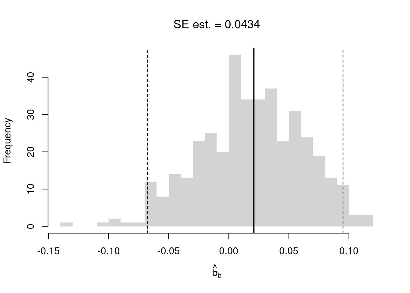
There are several resampling techniques. One main one is the bootstrap, which resamples with replacement for an arbitrary number of iterations. When bootstrapping a dataset with \(n\) observations, you randomly resample all \(n\) rows in your data set \(B\) times. We can then just take the percentiles of the bootstrap distribution.

# Original OLS coefficient
slope <-  coef(reg)[2]

# Bootstrap Sampling Distribution
boot_coefs <- rep(NA, 399)
for(i in seq_along(boot_coefs)){
    b_id <- sample( nrow(xy), replace=TRUE)
    xy_b <- xy[b_id, ]
    reg_b <- lm(y ~ x, data=xy_b)
    slope_b <- coef(reg_b)[2]
    boot_coefs[i] <- slope_b
}

# Plot Bootstrap Sampling Distribution
# + Percentile CI
hist(boot_coefs, breaks=25,
    main=NA, border=NA,
    freq=FALSE,
    xlab=expression(hat(b)[b]))
title('Bootstrap Distribution with 95% CIs', font.main=1)
boot_ci_percentile <- quantile(boot_coefs, probs=c(.025, .975))
abline(v=boot_ci_percentile, lty=2)

Normal Approximation with Jackknife SE.

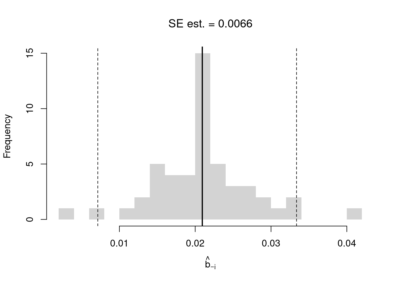
We also the jackknife, which loops through each row of the dataset. In each iteration of the loop, we drop that observation from the dataset and reestimate the statistic of interest. We then calculate the standard deviation of the statistic across all subsamples to get jackknife standard errors and, assuming the data are approximately normal, use Normal quantiles to construct a CI.¹

# Jackknife Sampling Distribution for OLS Coefficient
jack_coefs <- rep(NA, nrow(xy))
for(i in seq_along(jack_coefs)){
    xy_i <- xy[-i, ]
    reg_i <- lm(y ~ x, data=xy_i)
    slope_i <- coef(reg_i)[2]
    jack_coefs[i] <- slope_i
}
jack_se <- sd(jack_coefs)*sqrt(nrow(xy))

# Plot Estimated Sampling Distribution
x <- seq(-.2, +.25, by=.001)
fx <- dnorm(x, mean(jack_coefs), jack_se)
plot(x, fx, type='l', bty='n')
title('Normal Approx. with 95% CIs', font.main=1)

# Normal Approx Confidence Interval
jack_ci_normal <- qnorm(c(.025, .975), slope, jack_se)
abline(v=jack_ci_normal, lty=3)

# Bootstrap Quantiles
abline(v=boot_ci_percentile, lty=2)
legend('topright', lty=c(2,3), bty='n', cex=.75,
    title='Confidence Interval',
    legend=c('Bootstrap Percentile', 'Normal Approx.'))

13.3 Hypothesis Tests

We can also bootstrap other statistics, often to test a null hypothesis of “no relationship”. We are rarely interested in computing standard errors and conducting hypothesis tests for simple linear regressions in practice, but work through the ideas with two variables before moving to analyze multiple variables.

Invert a CI.

One main way to conduct hypothesis tests is to examine whether a confidence interval contains a hypothesized value. Does the slope coefficient equal \(0\)? For reasons we won’t go into in this class, we typically normalize the coefficient by its standard error: \(\hat{t} = \frac{\hat{b}}{\hat{s}_{\hat{b}}}\), where \(\hat{s}_{\hat{b}}\) is the estimated standard error of the coefficient.

# Create t-stat with jackknife SE
t_hat <- coef(reg)['x']/jack_se

boot_t <-  rep(NA, 399)
for(b in seq_along(boot_t)){
    # Bootstrap data
    b_id <- sample( nrow(xy), replace=TRUE)
    xy_b <- xy[b_id, ]
    # Redo regression
    reg_b <- lm(y ~ x, data=xy_b)
    slope_b <- coef(reg_b)[2]
    # Redo Jackknife SEs
    jack_coefs_b <- rep(NA, nrow(xy_b))
    for(i in seq_along(jack_coefs_b)){
        xy_b_i <- xy_b[-i, ]
        reg_b_i <- lm(y ~ x, data=xy_b_i)
        slope_b_i <- coef(reg_b_i)[2]
        jack_coefs_b[i] <- slope_b_i
    }
    jack_se_b <- sd(jack_coefs_b)*sqrt(nrow(xy_b))
    # Redo t with Jackknife SE
    t_hat_b <- slope_b/jack_se_b
    boot_t[b] <- t_hat_b
}

hist(boot_t, breaks=25,
    main=NA, border=NA, freq=FALSE,
    xlab=expression(hat(t)[b]),
    xlim=range(c(0, boot_t)) )
title('Bootstrap t with Jackknife SE', font.main=1)
abline(v=quantile(boot_t, probs=c(.025, .975)), lty=2)
abline(v=0, col=rgb(1, 0, 0, .8), lwd=2)

NoteMust Know

Suppose you have data on education level and wages. Conduct a linear regression. Then construct a \(95\%\) confidence interval for the slope coefficient and test the hypothesis of no relationship.

library(Ecdat)
xy <- Wages1[, c('school', 'wage')]

Impose the Null.

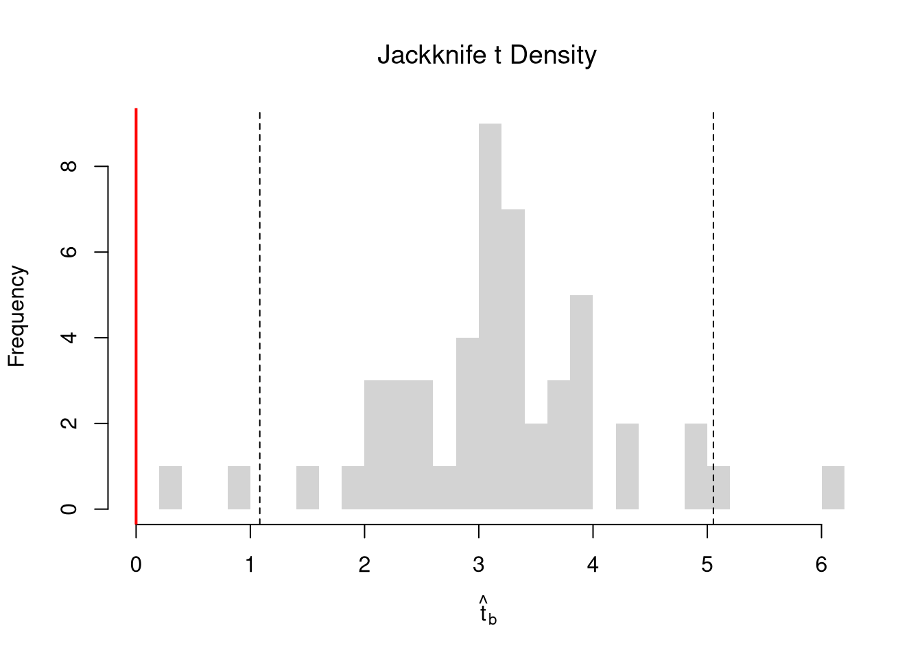
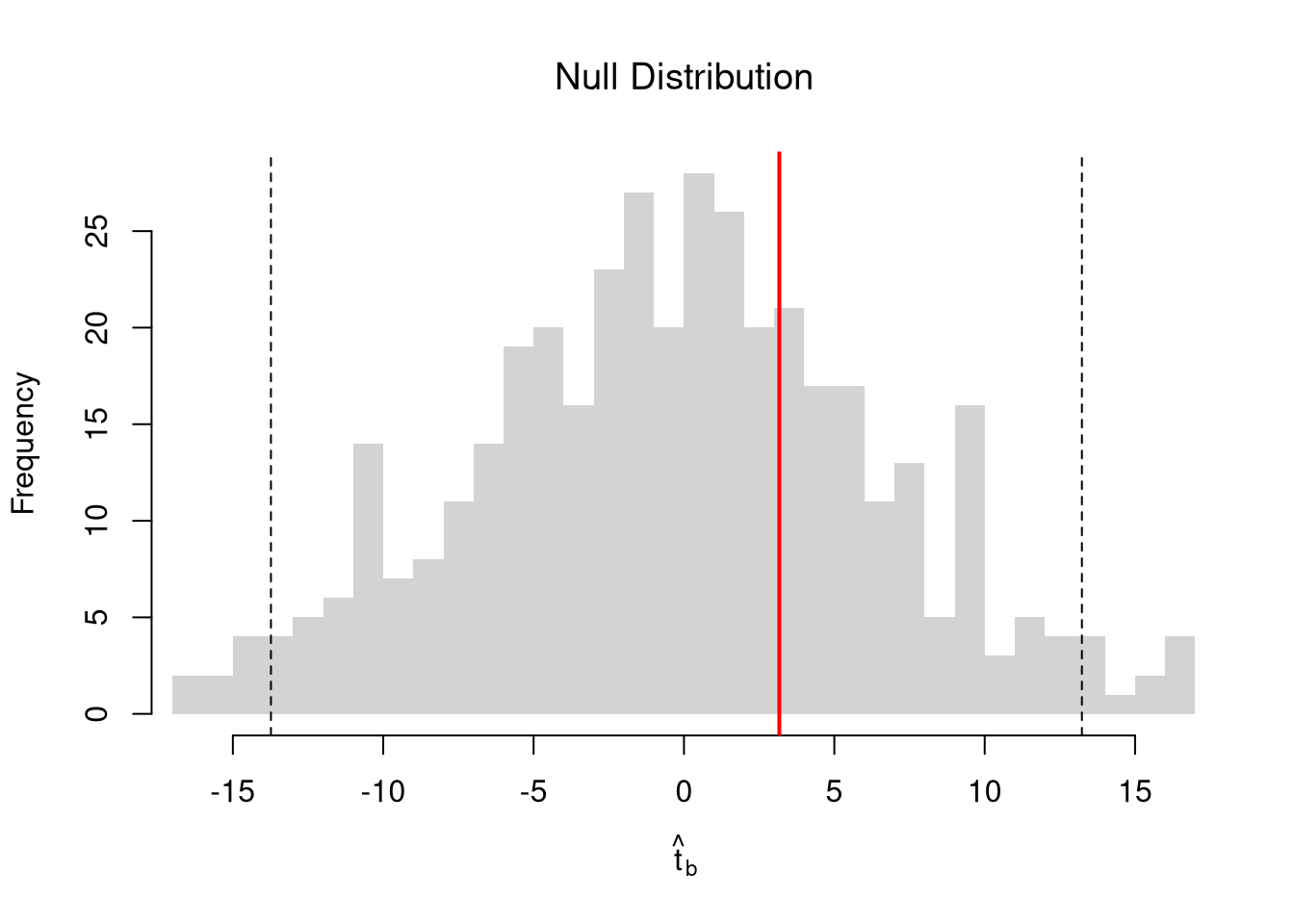
We can also compute a null distribution. We focus on the simplest: simulations that each impose the null hypothesis and re-estimate the statistic of interest. Specifically, we compute the distribution of \(t\)-values on data with randomly reshuffled outcomes (imposing the null), and compare how extreme the observed value is. We can sample with replacement (i.e., the null bootstrap) or without (permutation), just as with the correlation statistic.

# Null Distribution for Reg Coef
null_t <-  rep(NA, 399)
for(b in seq_along(null_t)){
    # Permuted data
    xy_b <- xy
    xy_b[, 'y'] <- sample( xy_b[, 'y'], replace=FALSE) #Bootstrap: replace=T
    reg_b <- lm(y ~ x, data=xy_b)
    # Redo regression
    reg_b <- lm(y ~ x, data=xy_b)
    slope_b <- coef(reg_b)[2]
    # Redo Jackknife SEs
    jack_coefs_b <- rep(NA, nrow(xy_b))
    for(i in seq_along(jack_coefs_b)){
        xy_b_i <- xy_b[-i, ]
        reg_b_i <- lm(y ~ x, data=xy_b_i)
        slope_b_i <- coef(reg_b_i)[2]
        jack_coefs_b[i] <- slope_b_i
    }
    # Redo t with Jackknife SE
    t_hat_b <- slope_b/ (sd(jack_coefs_b)*sqrt(nrow(xy_b)))
    null_t[b] <- t_hat_b
}

# Null Distribution
hist(null_t, breaks=25,
    main=NA, border=NA, freq=FALSE,
    xlab=expression(hat(t)[b]),
    xlim=range(null_t))
title('Null Distribution', font.main=1)
# 95% CI
null_ci <- quantile(null_t, probs=c(.025, .975))
abline(v=null_ci, lty=2)
# Observed value
abline(v=t_hat, col=rgb(1, 0, 0, .8), lwd=2)

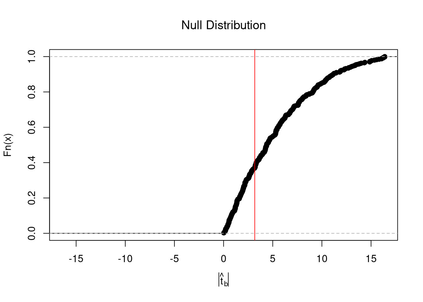
Permutations are common when testing against “no association”. From permuted data, we can calculate a \(p\)-value: the probability you would see something as at least as extreme as your statistic under the null (assuming your null hypothesis was true, see <01_08_HypothesisTests.qmd>). We calculate the \(p\)-value directly from the null distribution. Smaller \(p\)-values suggest more evidence against the null.

# Two Sided Test for P(t > jack_t or t < -jack_t | Null of t=0)
That_NullDist2 <- ecdf(abs(null_t))
Phat2  <-  1-That_NullDist2( abs(t_hat))
Phat2
## [1] 0.6340852
plot(That_NullDist2, xlim=range(null_t, t_hat),
    xlab=expression( abs(hat(t)[b]) ),
    main=NA)
title('Null Distribution', font.main=1)
abline(v=t_hat, col=rgb(1, 0, 0, .8))

TipTest Yourself

Interpret the \(p\)-value computed above. It is the fraction of the null distribution at least as extreme as the observed \(\hat{t}\). Suppose the code returned \(p=0.02\): in a world where the slope is truly zero, only \(2\%\) of samples would produce a \(|\hat{t}|\) this large, so under the common \(5\%\) rule (\(0.02 < 0.05\)) we reject the null of no relationship. A larger value such as \(p=0.30\) would mean such a \(\hat{t}\) is unremarkable under the null, so we would fail to reject.

# Hard decision rule at the 5% level
if(Phat2 < 0.05){
    'reject the null of no relationship'
} else {
    'fail to reject the null of no relationship'
}
## [1] "fail to reject the null of no relationship"

NoteMust Know

Suppose you have data on grades completed and wages. Conduct a linear regression. Then compute a \(p\)-value for the null hypothesis of no relationship between education level and wages.

library(Ecdat)
xy <- Wages1[, c('school', 'wage')]

Caveats.

We could also use hard decision rules, such as “\(p < 0.05\) is a statistically significant finding”. However, just like confidence intervals, those hard decision rules can be sensitive to somewhat arbitrary choices (Why Jackknife SE’s instead of classical ones? Why test at the \(95\%\) level rather than \(90\%\)?)

“No association” is the most common null hypothesis in practice, but we can also use bootstrapping to test against other specific hypothesis: \(\beta\), the population slope (formalized in Bivariate Probability). To impose the null in this case, you recenter the sampling distribution around the hypothetical value; \(\hat{t} = \frac{\hat{b} - \beta}{\hat{s}_{\hat{b}}}\).²

Although two-sided hypothesis tests are most common, you can also test one-sided hypotheses.

13.4 Association is not Causation

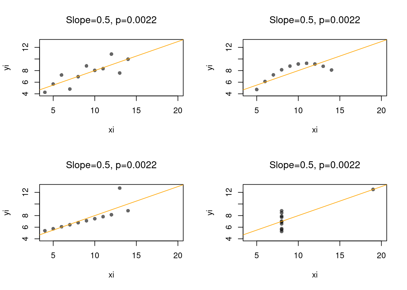
The same caveats about “correlation is not causation” extend to regression. You may be tempted to use the term “the effect”, but that interpretation of a regression coefficient assumes the linear model is true. If you fit a line to a non-linear relationship, then you will still get back a coefficient even though there is no singular the effect: the true relationship is non-linear! Also consider a classic example, Anscombe’s Quartet, which shows four very different datasets that give the same linear regression coefficient. Notice that you understand the problem because we used scatterplots to visual the data.³

# Anscombe's Quartet 

par(mfrow=c(2, 2))
for(i in 1:4){
    xi <- anscombe[, paste0('x', i)]
    yi <- anscombe[, paste0('y', i)]
    plot(xi, yi, ylim=c(4, 13), xlim=c(4, 20),
        pch=16, col=grey(0, .6), main=NA,
        xlab=paste0('x', i), ylab=paste0('y', i))
    reg <- lm(yi ~ xi)
    b <- round(coef(reg)[2], 2)
    p <- round(summary(reg)$coefficients[2, 4], 4)
    abline(reg, col=rgb(1, 0.6, 0, .8))
    title(paste0('Slope=', b, ', p=', p), font.main=1)
}

## For an even better example, see `Datasaurus Dozen'F
#browseURL(
#'https://bookdown.org/paul/applied-data-visualization/
#why-look-the-datasaurus-dozen.html')

It is true that linear regression “is the best linear predictor of the nonlinear regression function if the mean-squared error is used as the loss function” (Cameron and Trivedi 2005, 92). But this is not a carte-blanche justification for OLS, as the best of the bad predictors is still a bad predictor. For many economic applications, it is more helpful to think and speak of “dose response curves” instead of “the effect”.

While adding interaction terms or squared terms allows one incorporate heterogeneity and non-linearity, they change several features of the model (most of which are not intended). Often, there are nonsensical predicted values. For example, if the most of your age data are between \([23,65]\), a quadratic term can imply silly things for people aged \(10\) or \(90\).

Nonetheless, linear regression provides an important piece of quantitative information that is understood by many. All models are an approximation, and sometimes only unimportant nuances are missing from a vanilla linear model. Other times, that model can be seriously misleading. (This is especially true if your making policy recommendations based on a universal “the effect”.) As an exploratory tool, linear regession is a good guess but one whose point estimates should not be taken too seriously (in which case, the standard errors are also much less important). Before trying to find a regression specification that makes sense for the entire dataset, explore local relationships.

13.5 Exercises

1. Comment the script you wrote for this chapter, then restart R and check that it runs from a clean session, then check the script with AI as explained in Working with AI. Write three sentences from memory on the main statistical idea of this chapter, and ask the assistant what is wrong, vague, or missing. Finish with your own questions about whatever you found hardest.

2. Explain in words what the \(R^2\) statistic measures. A researcher runs a regression and finds \(\hat{R}^2 = 0.95\). Does this mean the model is correctly specified or that \(X\) causes \(Y\)? Why or why not?

3. Suppose you have \(n=4\) observations: \(\{(1, 3),\ (2, 5),\ (3, 6),\ (4, 10)\}\). Compute \(\hat{b}_0\) and \(\hat{b}_1\) by hand using \(\hat{b}_1 = \hat{C}_{XY}/\hat{V}_X\) and \(\hat{b}_0 = \hat{M}_Y - \hat{b}_1 \hat{M}_X\). Then compute the fitted values \(\hat{y}_i\), the residuals \(\hat{e}_i\), and \(\hat{R}^2\).

4. Using the mtcars dataset, regress mpg on wt with lm(). Report \(\hat{b}_0\), \(\hat{b}_1\), and \(\hat{R}^2\). Then write a bootstrap with \(B = 999\) iterations to construct a \(95\%\) percentile confidence interval for \(\hat{b}_1\) and check whether it contains zero.

Further Reading.

• https://www.econometrics-with-r.org/4-lrwor.html – OLS estimation, fitted values, and residuals explained step by step with R.
• https://learningstatisticswithr.com/book/regression.html – accessible introduction to simple linear regression including interpretation of coefficients and \(R^2\).
• https://www.khanacademy.org/math/statistics-probability/describing-relationships-quantitative-data/regression-library/v/introduction-to-residuals-and-least-squares-regression – video walkthrough of least-squares fitting and residual plots.

Recall

This chapter fit a single line to bivariate data: it derived the OLS slope \(\hat{b}_{1}=\hat{C}_{XY}/\hat{V}_{X}\) and intercept \(\hat{b}_{0}=\hat{M}_{Y}-\hat{b}_{1}\hat{M}_{X}\), measured goodness of fit with \(\hat{R}^{2}\), and built confidence intervals and \(p\)-values via the bootstrap, jackknife, and permutation. The three-observation worked example \(\{(1,2),(2,2.5),(3,4)\}\) traced through every step by hand and produced slope \(\hat{b}_{1}=1\), intercept \(\hat{b}_{0}=5/6\), \(\hat{TSS}=13/6\), \(\hat{RSS}=1/6\), and \(\hat{R}^{2}=12/13\approx 0.92\). The next chapter relaxes the single-slope assumption: bin the data and fit a separate local model in each bin, so the relationship can bend.

Cameron, A. C., and P. K. Trivedi. 2005. Microeconometrics: Methods and Applications. Cambridge University Press. https://books.google.de/books?id=Zf0gCwxC9ocC.

---

1. Recall that jackknife standard errors need to be rescaled because each jackknife resample is too similar to the next. For this reason, we also do not simply take the percentiles of the jackknife distribution. We can also calculate the standard deviation of the statistic across all bootstrap samples instead.

2. Under some additional assumptions, the null distribution follows a \(t\)-distribution. (For more on parametric t-testing based on statistical theory, see https://www.econometrics-with-r.org/4-lrwor.html.)

3. The same principles holds when comparing two groups: http://www.stat.columbia.edu/~gelman/research/published/causal_quartet_second_revision.pdf