Code
# Install R Data Package and Load in
install.packages('wooldridge') # only once
library('wooldridge') # "load" anytime you want to use the data
?wage1 # details about the dataset we want
head(wage1)Suppose our data is given in the table shown below.
| \(x=0\) | \(x=1\) | |
|---|---|---|
| \(y=1\) | \(12\) | \(8\) |
| \(y=2\) | \(18\) | \(6\) |
| \(y=3\) | \(10\) | \(16\) |
First, we can compute conditional probabilities to examine how the distribution changes.
| \(x=0\) | \(x=1\) | ||
|---|---|---|---|
| \(y=1\) | \(12/40\) | \(8/30\) | |
| \(y=2\) | \(18/40\) | \(6/30\) | |
| \(y=3\) | \(10/40\) | \(16/30\) | |
| \(40/40\) | \(30/30\) |
Second, we can compute the conditional mean \(\hat{M}_{Y|X}\) by looking within each row. Specifically \[\begin{eqnarray*} \hat{M}_{y|x=0} = 1 \frac{12}{40} + 2 \frac{18}{40} + 3 \frac{10}{40} = \frac{12+36+30}{40} = \frac{78}{40} \\ \hat{M}_{y|x=1} = 1 \frac{8}{30} + 2 \frac{6}{30} + 3 \frac{16}{30} = \frac{8+12+48}{30} = \frac{68}{30} \end{eqnarray*}\] Notice that \(\hat{M}_{y|x=0} < 2 < \hat{M}_{y|x=1}\), which shows that the mean value of \(Y\) is higher when \(X\) is higher. I.e., there is a positive association.
For mixed data, \(\hat{Y}_{i}\) is a cardinal variable and \(\hat{X}_{i}\) is a factor variable (typically unordered). For such “grouped data”, we analyze associations via group comparisons. The basic idea is best seen in a comparison of two samples, which corresponds to an \(\hat{X}_{i}\) with two categories. For example, the heights of men and women in Canada or the homicide rates in two different American states.
We will consider the wages for people with and without completing a degree. To have this data on our computer, we must first install the “wooldridge” package once. Then we can access the data at any time by loading the package.
# Install R Data Package and Load in
install.packages('wooldridge') # only once
library('wooldridge') # "load" anytime you want to use the data
?wage1 # details about the dataset we want
head(wage1)To compare wages for people with and without completing a degree, we start by making a histogram for both groups.
library('wooldridge')
## Wages
Y <- wage1[, 'wage']
## Group 1: Not Graduates
X1_id <- wage1[,'educ'] == 15
Y1 <- Y[X1_id]
## Group 2: Graduates
X2_id <- wage1[,'educ'] == 16
Y2 <- Y[X2_id]


# Initial Summary Figure
bks <- seq(0, 24, by=1.5)
dlim <- c(0,.2)
cols <- c(rgb(1,0,0,.5), rgb(0,0,1,.5))

hist(Y1, breaks=bks, ylim=dlim,
     col=cols[1], xlab='Wages',
     freq=F, border=NA, main='')
hist(Y2, breaks=bks, ylim=dlim,
     col=cols[2],
     freq=F, border=NA, add=T)
legend('topright',
       col=cols, pch=15,
       legend=c('15 Years', '16 Years'),
       title='School Completed')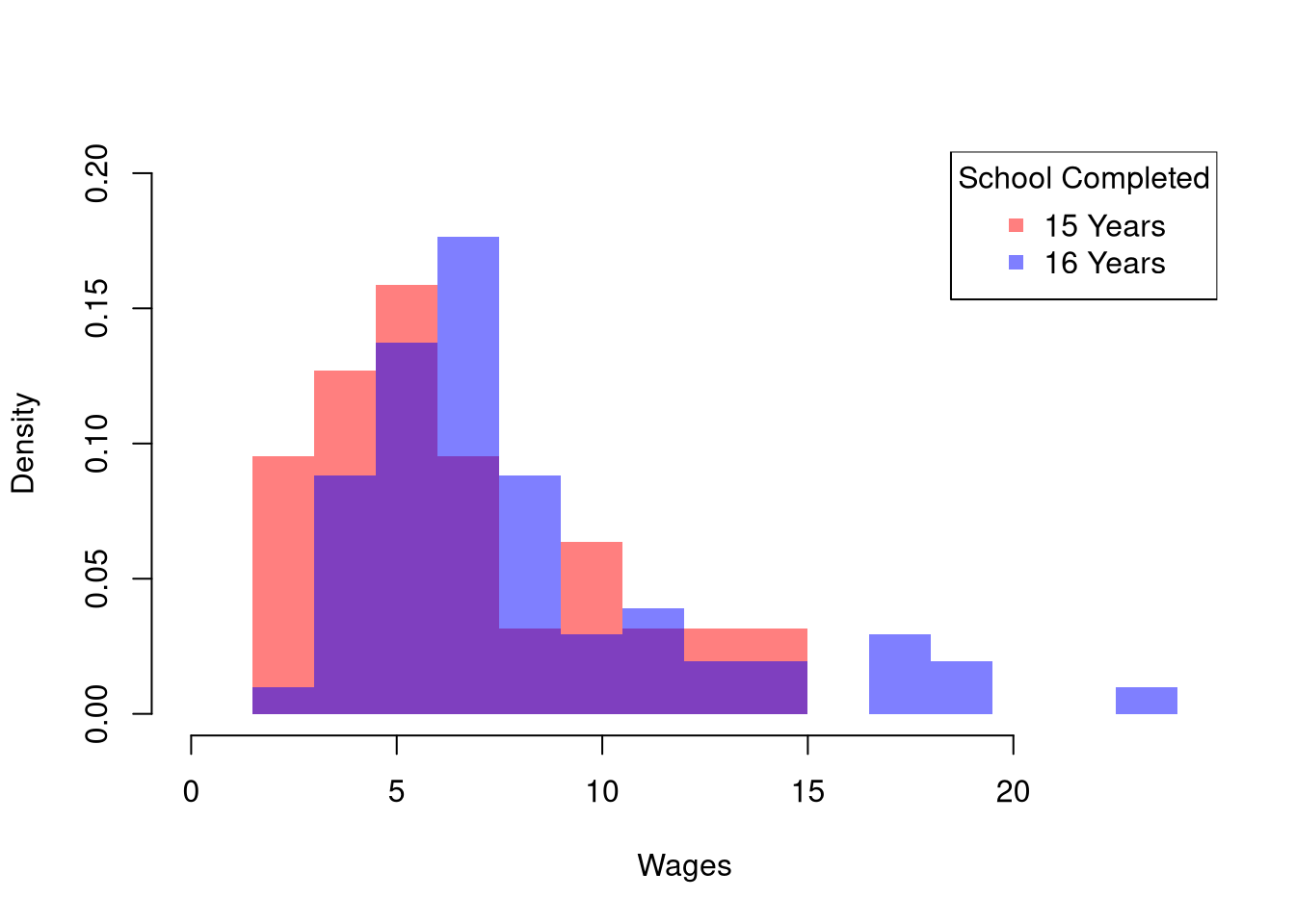
The histogram may show several differences between groups or none at all. Often, the first statistic we investigate for hypothesis testing is the mean.
We often want to know if the means of different samples are the same or different. To test this hypothesis, we compute the means separately for each sample and then examine the differences term \[\begin{eqnarray} \hat{D} = \hat{M}_{Y1} - \hat{M}_{Y2}, \end{eqnarray}\] with a null hypothesis that there is no difference in the population means. We can do this either by “inverting a Confidence Interval” or “imposing the null”.
Here is an example of inverting a CI
# Differences between means
m1 <- mean(Y1)
m2 <- mean(Y2)
d <- m1-m2

# Bootstrap Distribution
bootstrap_diff <- vector(length=9999)
for(b in seq(bootstrap_diff) ){
    Y1_b <- sample(Y1, replace=T)
    Y2_b <- sample(Y2, replace=T)
    m1_b <- mean(Y1_b)
    m2_b <- mean(Y2_b)
    d_b <- m1_b - m2_b
    bootstrap_diff[b] <- d_b
}
hist(bootstrap_diff,
    border=NA, font.main=1,
    main='Bootstrapped Difference in Means')

# 2-Sided Test via Confidence Interval
boot_ci <- quantile(bootstrap_diff, probs=c(.025, .975))
abline(v=boot_ci, lwd=2)
abline(v=0, lwd=2, col=2)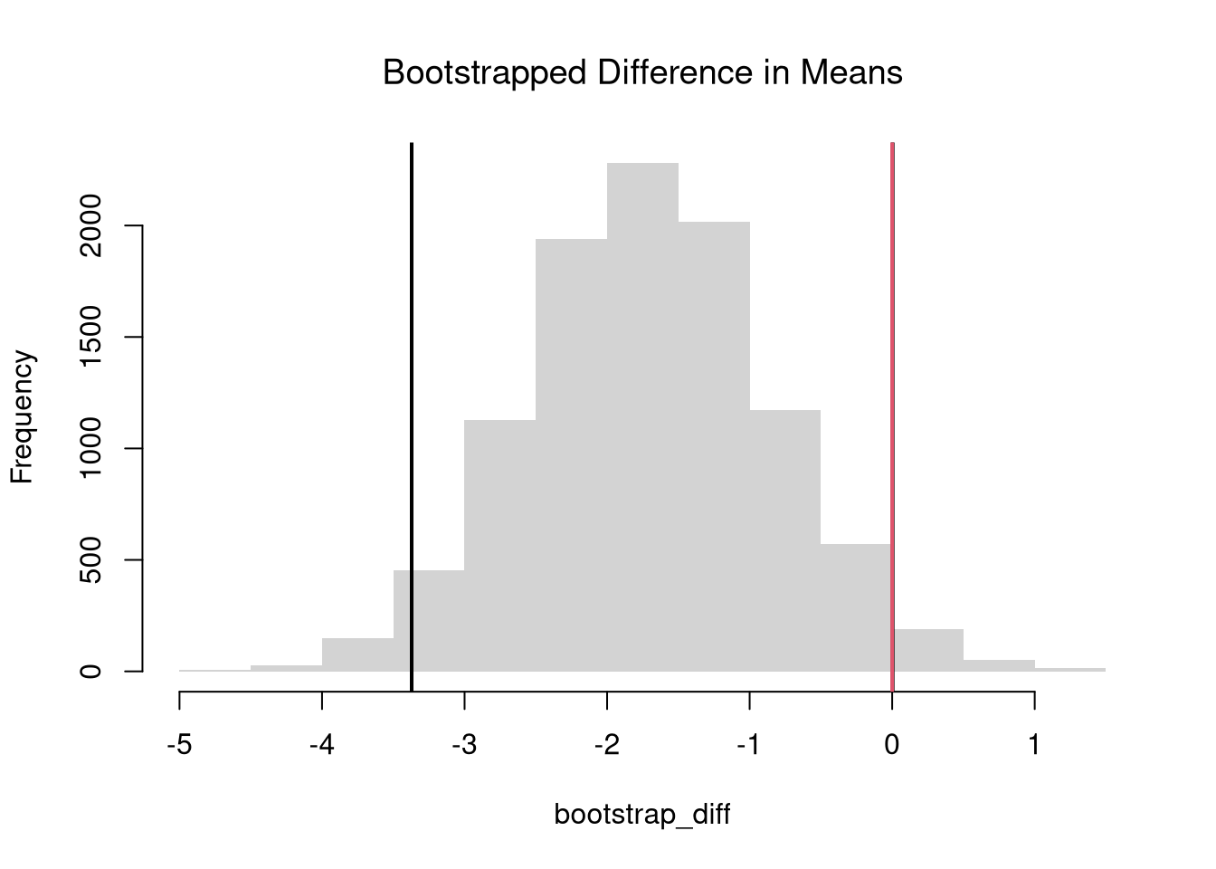
For “imposing the null”, it is more common to use \(p\)-values instead of confidence intervals. We can compute \(p\)-values using a null-bootstrap or permutation distribution. If using a hard decision rule, it is most common to use
# Null Bootstrap Distribution
permute_diff <- vector(length=9999)
for(b in seq(permute_diff) ){
    #randomize data
    Y_b  <- sample(Y, replace=F)
    Y1_b <- Y_b[X1_id]
    Y2_b <- Y_b[X2_id]
    # recompute statistic
    m1_b <- mean(Y1_b)
    m2_b <- mean(Y2_b)
    d_b <- m1_b - m2_b
    permute_diff[b] <- d_b
}
hist(permute_diff,
    border=NA, font.main=1,
    main='Permuted Difference in Means')
abline(v=d, col=2)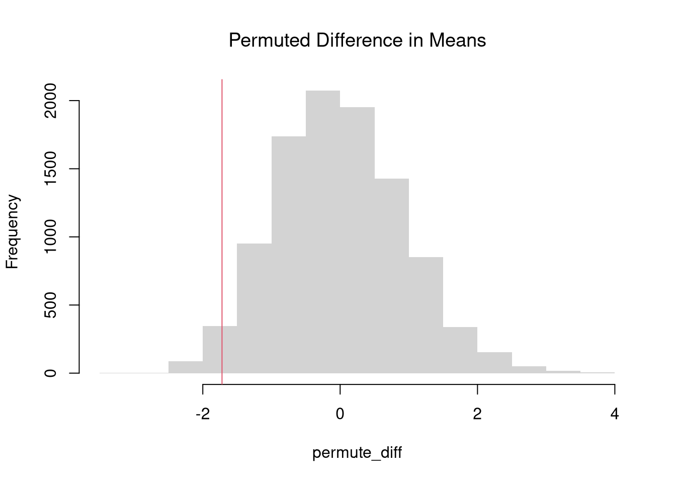
Fhat_abs0 <- ecdf(abs(permute_diff))
p <- 1 - Fhat_abs0( abs(d) )
p
## [1] 0.06380638
Those are purely statistical statements that only speak to how frequent differences are generated by random chance. They do not say why there are any differences or how large they are. Even on purely statistical grounds, however, we would want to be cautious about a making data-driven decisions when
For such reasons, applied statisticians consider many statistics
The above procedure generalized from differences in means to other quantiles statistics like medians. To start, we plot the ECDF’s for both groups.
# Quantile Comparison

## Distribution 1
F1 <- ecdf(Y1)
plot(F1, col=cols[1],
     pch=16, xlab='Wages', xlim=c(0,24),
     main='Comparing Medians',
     font.main=1, bty='n')
## Median 1
med1 <- quantile(F1, probs=0.5)
segments(med1, 0, med1, 0.5, col=cols[1], lty=2)
abline(h=0.5, lty=2)

## Distribution 2
F2 <- ecdf(Y2)
plot(F2, add=TRUE, col=cols[2], pch=16)
## Median 2
med2 <- quantile(F2, probs=0.5)
segments(med2, 0, med2, 0.5, col=cols[2], lty=2)

## Legend
legend('bottomright',
       col=cols, pch=15,
       legend=c('Grade 15', 'Grade 16'),
       title='School Completed')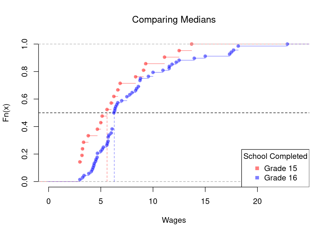
# Bootstrap Distribution Function
boot_quant <- function(Y1, Y2, B=9999, probs=0.5, ...){
    bootstrap_diff <- vector(length=B)
    for(b in seq(bootstrap_diff)){
        Y1_b <- sample(Y1, replace=T)
        Y2_b <- sample(Y2, replace=T)
        q1_b <- quantile(Y1_b, probs=probs, ...)
        q2_b <- quantile(Y2_b, probs=probs, ...)
        d_b <- q1_b - q2_b
        bootstrap_diff[b] <- d_b
    }
    return(bootstrap_diff)
}

# 2-Sided Test for Median Differences
# d <- quantile(Y2, probs=0.5) - quantile(Y1, probs=0.5)
boot_d <- boot_quant(Y1, Y1, B=999, probs=0.5)
hist(boot_d, border=NA, font.main=1,
    main='Bootstrap Difference in Medians')
abline(v=quantile(boot_d, probs=c(.025, .975)), lwd=2)
abline(v=0, lwd=2, col=2)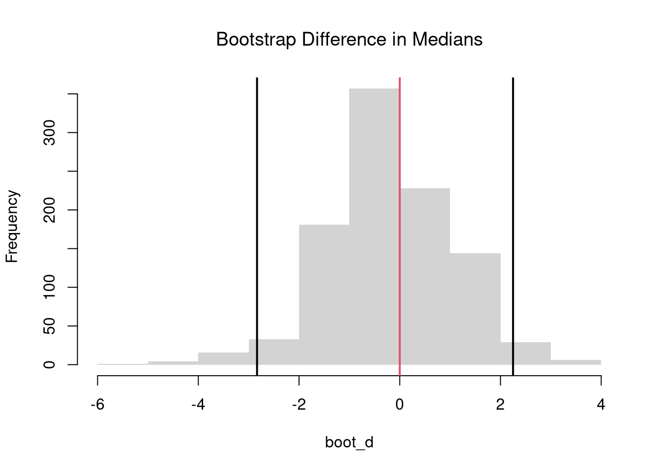
The above procedure is quite general and extends to other quantiles. Note that bootstrap tests can perform poorly with highly unequal variances or skewed data. To see this yourself, make a simulation with skewed data and unequal variances.
In principle, we can also examine whether there are differences in spread (sd or IQR) or shape (skew or kurtosis). We use the same hypothesis testing procedure as above
We can also examine whether there are any differences between the entire distributions. We typically start by plotting the data using ECDF’s or a boxplot, and then calculate a statistic for hypothesis testing. Which plot and test statistic depends on how many groups there are.
One useful visualization for two groups is to plot the quantiles against one another: a quantile-quantile plot. I.e., the first data point on the bottom left shows the first quantile for both distributions.
# Wage Data (same as from before)
#library(wooldridge)
#Y1 <- sort( wage1[wage1[,'educ'] == 15,  'wage'])
#Y2 <- sort( wage1[wage1[,'educ'] == 16,  'wage'] )

# Compute Quantiles
quants <- seq(0,1,length.out=101)
Q1 <- quantile(Y1, probs=quants)
Q2 <- quantile(Y2, probs=quants)

# Compare Distributions via Quantiles
#ry <- range(c(Y1, Y2))
#plot(ry, c(0,1), type='n', font.main=1,
#    main='Distributional Comparison',
#    xlab="Quantile",
#    ylab="Probability")
#lines(Q1, quants, col=2)
#lines(Q2, quants, col=4)
#legend('bottomright', col=c(2,4), lty=1,
#   legend=c(
#       expression(hat(F)[1]),
#       expression(hat(F)[2])
#))

# Compare Quantiles
ry <- range(c(Y1, Y2))
plot(Q1, Q2, xlim=ry, ylim=ry,
    xlab=expression(Q[1]),
    ylab=expression(Q[2]),
    main='Quantile-Quantile Plot',
    font.main=1,
    pch=16, col=grey(0,.25))
abline(a=0,b=1,lty=2)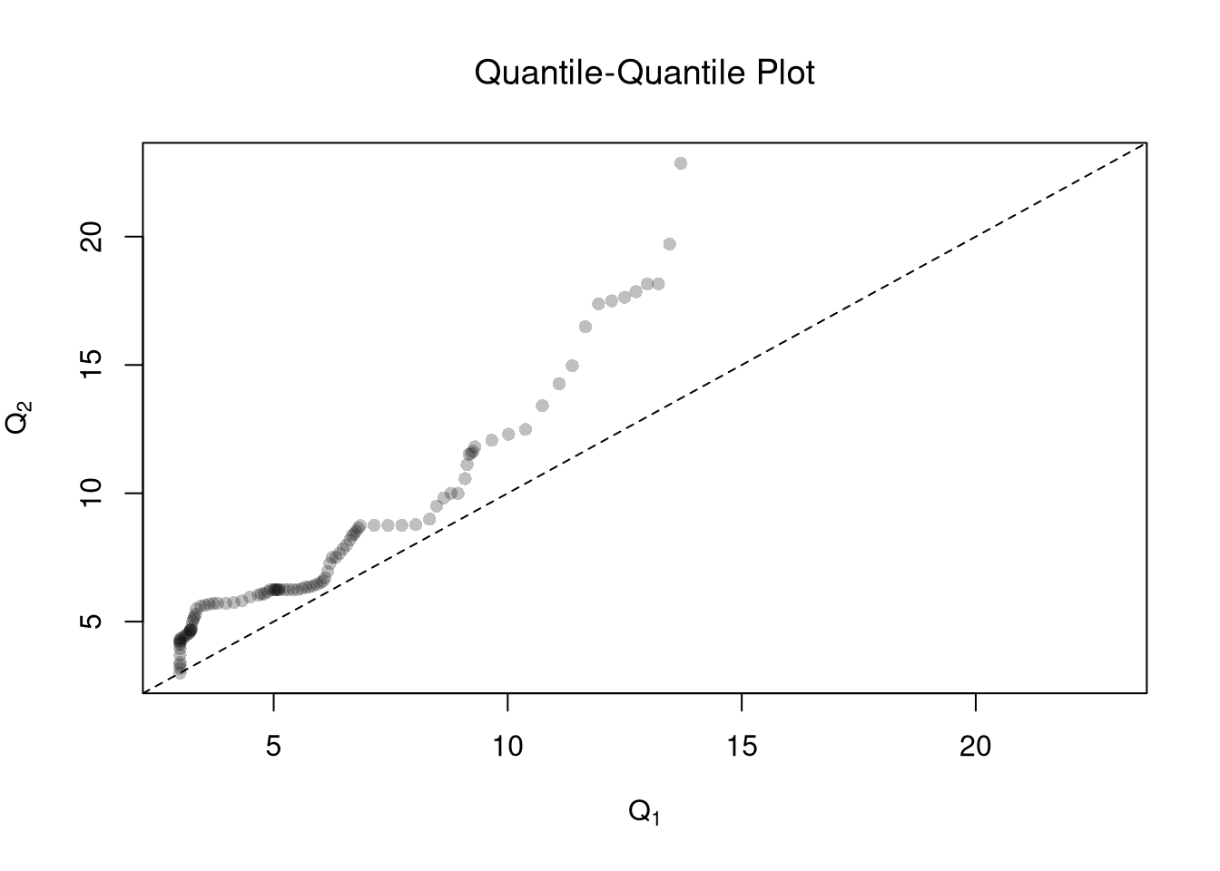
The starting point for hypothesis testing is the Kolmogorov-Smirnov Statistic: the maximum absolute difference between two CDF’s over all sample data \(y \in \{Y_1\} \cup \{Y_2\}\). \[\begin{eqnarray} \hat{KS} &=& \max_{y} |\hat{F}_{1}(y)- \hat{F}_{2}(y)|^{p}, \end{eqnarray}\] where \(p\) is an integer (typically 1). An intuitive alternative is the Cramer-von Mises Statistic: the sum of absolute differences (raised to an integer, typically 2) between two CDF’s. \[\begin{eqnarray} \hat{CVM} &=& \sum_{y} | \hat{F}_{1}(y)- \hat{F}_{2}(y)|^{p}. \end{eqnarray}\]
# Distributions
y <- sort(c(Y1, Y2))
F1 <- ecdf(Y1)(y)
F2 <- ecdf(Y2)(y)

library(twosamples)

# Kolmogorov-Smirnov
KSq <- which.max(abs(F2 - F1))
KSqv <- round(twosamples::ks_stat(Y1, Y2),2)

# Cramer-von Mises Statistic (p=2)
CVMqv <- round(twosamples::cvm_stat(Y1, Y2, power=2), 2)

# Visualize Differences
plot(range(y), c(0,1), type="n", xlab='x', ylab='ECDF')
lines(y, F1, col=cols[1], lwd=2)
lines(y, F2, col=cols[2], lwd=2)

# KS
title( paste0('KS: ', KSqv), adj=0, font.main=1)
segments(y[KSq], F1[KSq], y[KSq], F2[KSq], lwd=1.5, col=grey(0,.75), lty=2)

# CVM
title( paste0('CVM: ', CVMqv), adj=1, font.main=1)
segments(y, F1, y, F2, lwd=.5, col=grey(0,.2))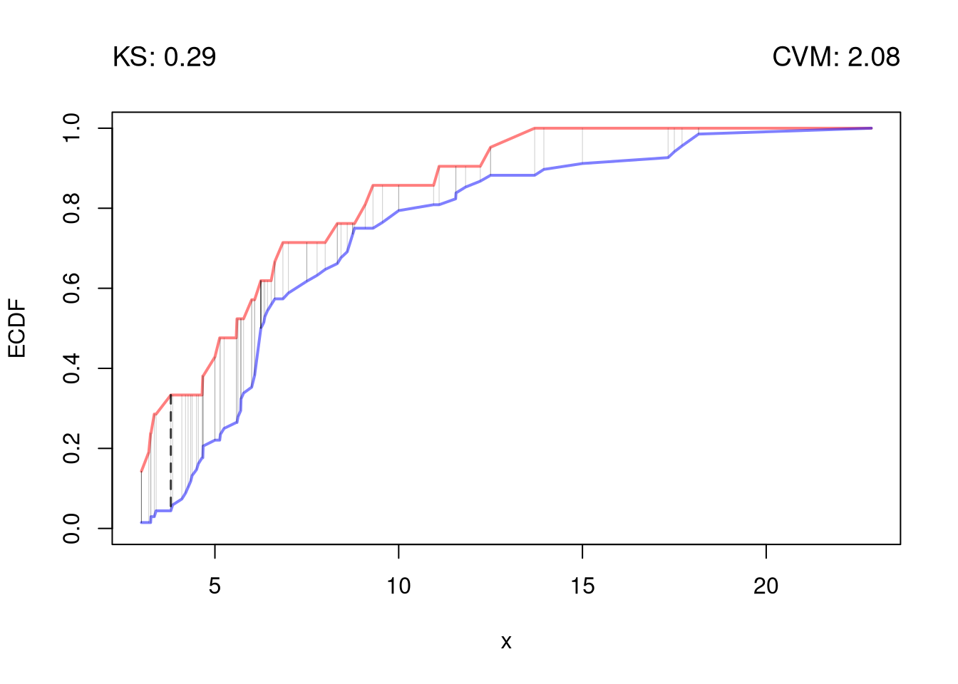
Just as before, you use bootstrapping for hypothesis testing.
twosamples::ks_test(Y1, Y2)
## Test Stat   P-Value
## 0.2892157 0.0940000

twosamples::cvm_test(Y1, Y2)
## Test Stat   P-Value
## 2.084253 0.083000With multiple groups, you will want to begin with a summary figure (such as a boxplot). We can also tests the equality of all distributions (whether at least one group is different). The Kruskal-Wallis test examines \(H_0:\; F_1 = F_2 = \dots = F_G\) versus \(H_A:\) at least one \(F_g\) differs, where \(F_g\) is the continuous distribution of group \(g=1,...G\). This test does not tell us which group is different.
To conduct the test, first denote individuals \(i=1,...n\) with overall ranks \(\hat{r}_1,....\hat{r}_{n}\). Each individual belongs to group \(g=1,...G\), and each group \(g\) has \(n_{g}\) individuals with average rank \(\bar{r}_{g} = \sum_{i} \hat{r}_{i} /n_{g}\). The Kruskal Wallis statistic is \[\begin{eqnarray} \hat{KW} &=& (n-1) \frac{\sum_{g=1}^{G} n_{g}( \bar{r}_{g} - \bar{r} )^2 }{\sum_{i=1}^{n} ( \hat{r}_{i} - \bar{r} )^2}, \end{eqnarray}\] where \(\bar{r} = \frac{n+1}{2}\) is the grand mean rank.
In the special case with only two groups, the Kruskal Wallis test reduces to the Mann–Whitney U test (also known as the Wilcoxon rank-sum test). In this case, we can write the hypotheses in terms of individual outcomes in each group, \(Y_i\) in one group \(Y_j\) in the other; \(H_0: Prob(Y_i > Y_j)=Prob(Y_i > Y_i)\) versus \(H_A: Prob(Y_i > Y_j) \neq Prob(Y_i > Y_j)\). The corresponding test statistic is \[\begin{eqnarray} \hat{U} &=& \min(\hat{U}_1, \hat{U}_2) \\ \hat{U}_g &=& \sum_{i\in g}\sum_{j\in -g} \Bigl[\mathbf 1( \hat{Y}_{i} > \hat{Y}_{j}) + \tfrac12\mathbf 1(\hat{Y}_{i} = \hat{Y}_{j})\Bigr]. \end{eqnarray}\]
A practical workflow for multiple groups has three steps:
# Built-in dataset with 6 groups
dat <- InsectSprays

# Step 1: Visual summary
boxplot(count~spray, data=dat,
    col=hcl.colors(6, alpha=.45),
    ylab="Insect count", xlab="Spray", main="")
title("Multiple-group comparison", font.main=1)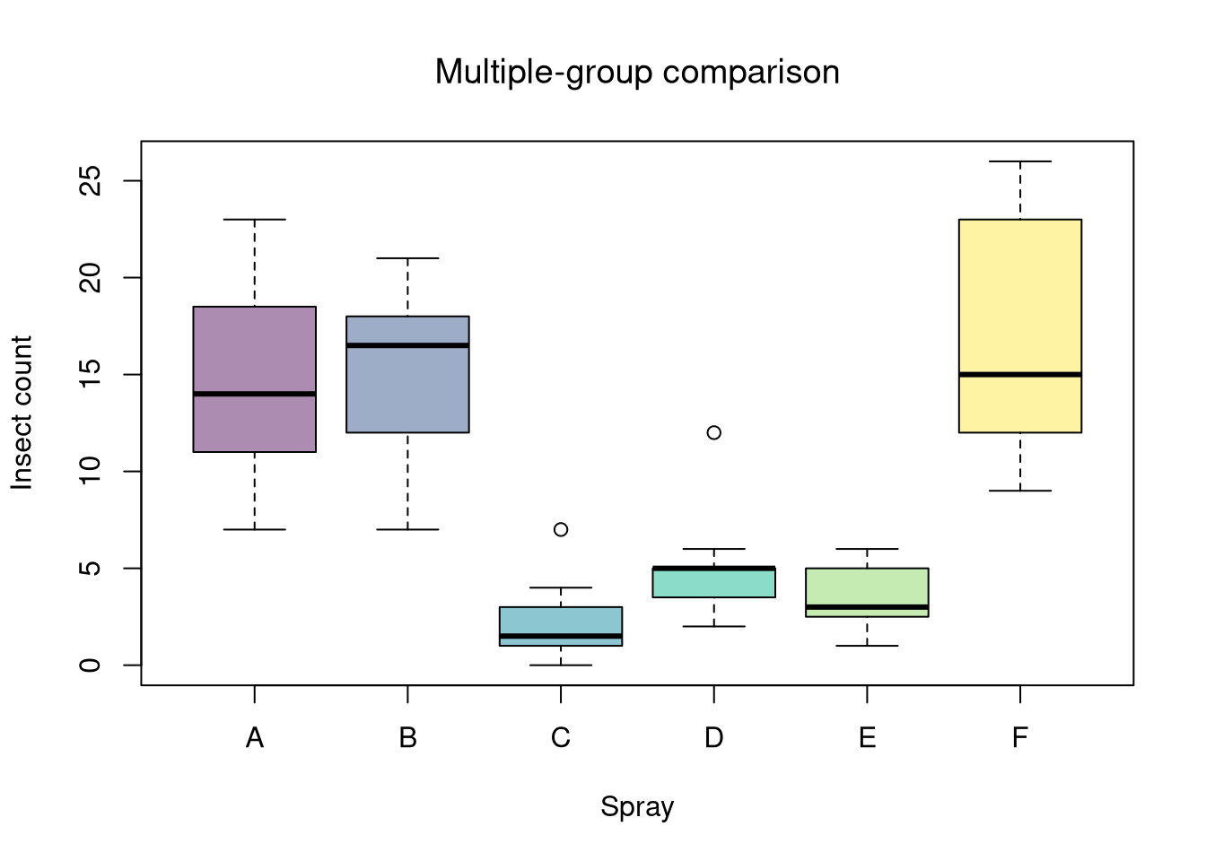
# Step 2: Global null test
kw <- kruskal.test(count~spray, data=dat)
kw
##
##  Kruskal-Wallis rank sum test
##
## data:  count by spray
## Kruskal-Wallis chi-squared = 54.691, df = 5, p-value = 1.511e-10

# Step 3: Post-hoc pairwise tests, adjusted p-values
pw <- pairwise.wilcox.test(
    x = dat$count, g = dat$spray,
    p.adjust.method = "bonferroni")
pw$p.value
##              A            B           C           D           E
## B 1.0000000000           NA          NA          NA          NA
## C 0.0005754382 0.0005754382          NA          NA          NA
## D 0.0011675305 0.0010374559 0.039766223          NA          NA
## E 0.0005092504 0.0005092504 0.788601898 1.000000000          NA
## F 1.0000000000 1.0000000000 0.000515337 0.001048967 0.000515337
Interpretation template:
library(Ecdat)
data(Caschool)
Caschool[,'stratio'] <- Caschool[,'enrltot']/Caschool[,'teachers']

# Do student/teacher ratio differ for at least 1 county?
# Single test of multiple distributions
library(coin)
kruskal_test(stratio~county, Caschool, distribution='approximate')Other Statistics