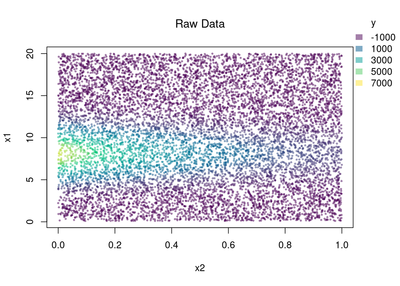
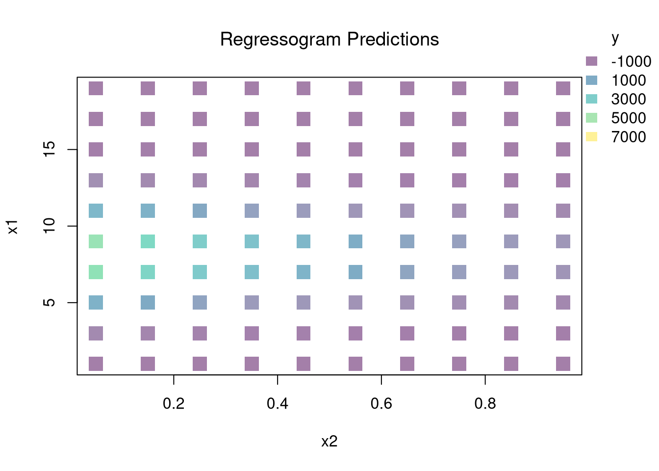
You can estimate a nonparametric model with multiple \(X\) variables with a multivariate regressogram. Here, we cut the data into exclusive bins along each dimension (called dummy variables), and then run a regression on all dummy variables.
################### Multivariate Regressogram#################### Regressogram Binsdat$x1c <-cut(dat$x1, bks1)#head(dat$x1c,3)dat$x2c <-cut(dat$x2, bks2)## Regressogramreg <-lm(y~x1c*x2c, data=dat) #nonlinear w/ complex interactions## Predicted Values## For Points in Middle of Each Binpred_df_rgrm <-expand.grid(x1c=levels(dat$x1c),x2c=levels(dat$x2c))pred_df_rgrm$yhat <-predict(reg, newdata=pred_df_rgrm)pred_df_rgrm <-cbind(pred_df_rgrm, pred_x)## Plot Predictionspar(oma=c(0,0,0,2))plot(x1~x2, pred_df_rgrm,col=ycol_pal[cut(pred_df_rgrm$yhat,col_scale)],pch=15, cex=2,main='Regressogram Predictions', font.main=1)add_legend(x='topright', col_scale=col_scale,yl=6, inset=c(0,.05),title='y')
21.2 Local Regressions
Just like with bivariate data, you can also use split-sample (or peicewise) regressions for multivariate data.
Break Points.
Incorporating Kinks and Discontinuities in \(X\) are a type of transformation that can be modeled using factor variables. As such, \(F\)-tests can be used to examine whether a breaks is statistically significant.
Code
library(Ecdat)data(Caschool)Caschool$score <- (Caschool$readscr + Caschool$mathscr) /2reg <-lm(score~avginc, data=Caschool)# F Test for Breakreg2 <-lm(score ~ avginc*I(avginc>15), data=Caschool)anova(reg, reg2)# Chow Test for Breakdata_splits <-split(Caschool, Caschool$avginc <=15)resids <-sapply(data_splits, function(dat){ reg <-lm(score ~ avginc, data=dat)sum( resid(reg)^2)})Ns <-sapply(data_splits, function(dat){ nrow(dat)})Rt <- (sum(resid(reg)^2) -sum(resids))/sum(resids)Rb <- (sum(Ns)-2*reg$rank)/reg$rankFt <- Rt*Rbpf(Ft,reg$rank, sum(Ns)-2*reg$rank,lower.tail=F)# See also# strucchange::sctest(y~x, data=xy, type="Chow", point=.5)# strucchange::Fstats(y~x, data=xy)# To Find Changes# segmented::segmented(reg)
21.3 Model Selection
One of the most common approaches to selecting a model or bandwidth is to minimize error. Leave-one-out Cross-validation minimizes the average “leave-one-out” mean square prediction errors: \[\begin{eqnarray}
\min_{\mathbf{H}} \quad \frac{1}{n} \sum_{i=1}^{n} \left[ \hat{Y}_{i} - \hat{y_{[i]}}(\mathbf{X},\mathbf{H}) \right]^2,
\end{eqnarray}\] where \(\hat{y}_{[i]}(\mathbf{X},\mathbf{H})\) is the model predicted value at \(\mathbf{X}_{i}\) based on a dataset that excludes \(\mathbf{X}_{i}\), and \(\mathbf{H}\) is matrix of bandwidths. With a weighted least squares regression on three explanatory variables, for example, the matrix is \[\begin{eqnarray}
\mathbf{H}=\begin{pmatrix}
h_{1} & 0 & 0 \\
0 & h_{2} & 0 \\
0 & 0 & h_{3} \\
\end{pmatrix},
\end{eqnarray}\] where each \(h_{k}\) is the bandwidth for variable \(X_{k}\).
There are many types of cross-validation . For example, one extension is k-fold cross validation, which splits \(N\) datapoints into \(k=1...K\) groups, each sized \(B\), and predicts values for the left-out group. adjusts for the degrees of freedom, whereas the function in R uses by default. You can refer to extensions on a case by case basis.
21.4 Hypothesis Testing
There are two main ways to summarize gradients: how \(Y\) changes with \(X\).
For regressograms, you can approximate gradients with small finite differences. For some small \(h_{p}\), we can compute \[\begin{eqnarray}
\hat{\beta}_{p}(\mathbf{x}) &=& \frac{ \hat{y}(x_{1},...,x_{p}+ \frac{h_{p}}{2}...,x_{P})-\hat{y}(x_{1},...,x_{p}-\frac{h_{p}}{2}...,x_{P})}{h_{p}},
\end{eqnarray}\]
When using split-sample regressions or local linear regressions, you can use the estimated slope coefficients \(\hat{\beta}_{p}(\mathbf{x})\) as gradient estimates in each direction.
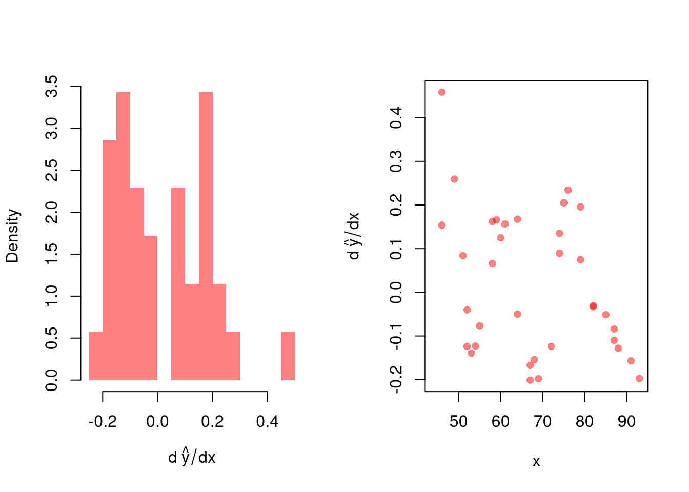
After computing gradients, you can summarize them in various plots: Histogram of \(\hat{\beta}_{p}(\mathbf{x})\), Scatterplot of \(\hat{\beta}_{p}(\mathbf{x})\) vs. \(X_{p}\), or the CI of \(\hat{\beta}_{p}(\mathbf{x})\) vs \(\hat{\beta}_{p}(\mathbf{x})\) after sorting the gradients
You may also be interested in a particular gradient or a single summary statistic. For example, a bivariate regressogram can estimate the marginal effect of \(X_{1}\) at the means; \(\hat{\beta_{1}}(\bar{\mathbf{x}}=[\bar{x_{1}}, \bar{x_{2}}])\). You may also be interested in the mean of the marginal effects (sometimes said simply as “average effect”), which averages the marginal effect over all datapoints in the dataset: \(1/n \sum_{i}^{n} \hat{\beta_{1}}(\mathbf{X}_{i})\), or the median marginal effect. Such statistics are single numbers that can be presented similar to an OLS regression table where each row corresponds a variable and each cell has two elements: “mean gradient (sd gradient)”.
Example with Bivariate Data.
Often, we are interested in gradients: how \(Y\) changes with \(X\). The linear model depicts this as a simple constant, \(\hat{b}_{1}\), whereas other models do not. A great first way to assess gradients is to plot the predicted values over the explanatory values.
More formally, there are two ways to summarize gradients
For all methods, including regressograms, you can approximate gradients with small finite differences. For some small difference \(d\), we can manually compute \[\begin{eqnarray}
\hat{b}_{1}(x) &=& \frac{ \hat{y}(x+\frac{d}{2}) - \hat{y}(x-\frac{d}{2})}{d},
\end{eqnarray}\]
When using split-sample regressions or local linear regressions, you can use the estimated slope coefficients \(\hat{b}_{1}(x)\) as gradient estimates in each direction.
After computing gradients, you can summarize them in various plots
You may also be interested in a particular gradient or a single summary statistic. For example, a bivariate regressogram can estimate the “marginal effect at the mean”; \(\hat{b}_{1}( x=\hat{M}_{X} )\). More typically, you would be interested in the “mean of the gradients”, sometimes said simply as “average effect”, which averages the gradients over all datapoints in the dataset: \(1/n \sum_{i}^{n} \hat{b}_{1}(x=\hat{X}_{i})\). Alternatively, you may be interested in the median of the gradients, or measures of “effect heterogeneity”: the interquartile range or standard deviation of the gradients. Such statistics are single numbers that can be presented in tabular form: “mean gradient (sd gradient)”. You can alternative report standard errors: “mean gradient (estimated se), sd gradient (estimated se)”.
Code
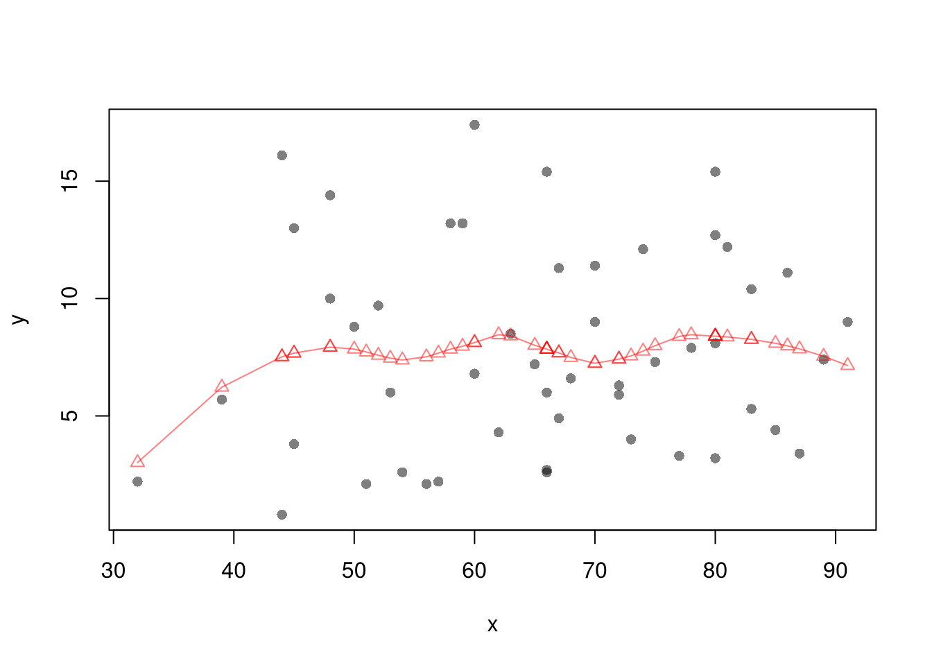
## Tabular Summarytab_stats <-c(M=mean(grad_lo, na.rm=T),S=sd(grad_lo, na.rm=T))tab_stats## M S ## 0.01554515 0.16296598## Use bootstrapping to get SE'sboot_stats <-matrix(NA, nrow=299, ncol=2)colnames(boot_stats) <-c('M se', 'S se')for(b in1:nrow(boot_stats)){ xy_b <- xy0[sample(1:nrow(xy0), replace=T),] reg_lo <-loess(y~x, data=xy_b, span=.6) pred_lo <-predict(reg_lo) grad_lo <-diff(pred_lo)/diff(xy_b[,'x']) dydx_mean <-mean(grad_lo, na.rm=T) dydx_sd <-sd(grad_lo, na.rm=T) boot_stats[b,1] <- dydx_mean boot_stats[b,2] <- dydx_sd}apply(boot_stats, 2, sd)## M se S se ## 0.04722890 0.06431175
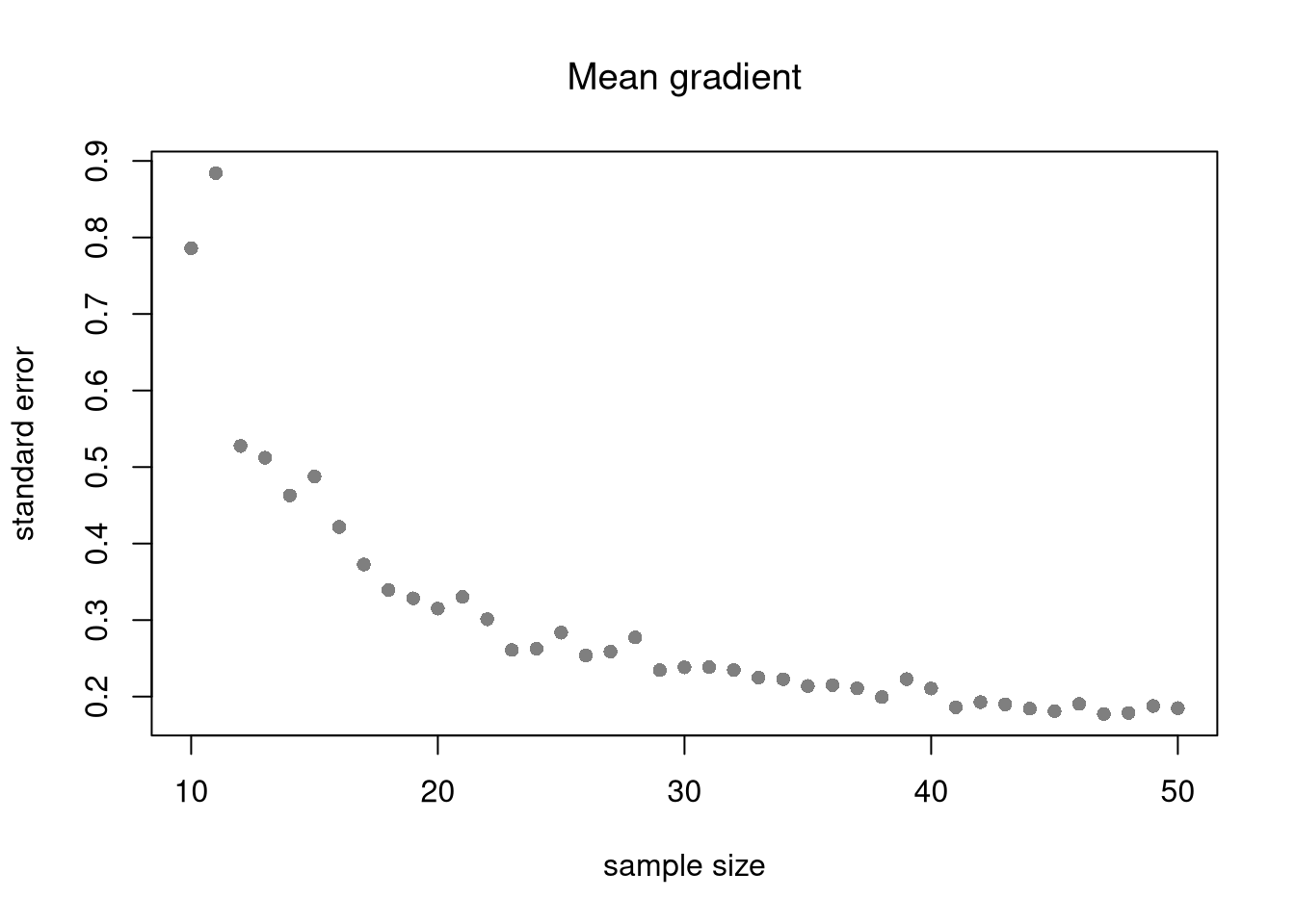
Diminishing Returns.
Just as before, there are diminishing returns to larger sample sizes for bivariate statistics. For example, the slope coefficient in simple OLS varies less from sample to sample when the samples are larger. Same for the gradients in loess. This decreased variability across samples makes hypothesis testing more accurate.
Code
B <-300Nseq <-seq(10,50, by=1)SE <-sapply(Nseq, function(n){ sample_stat <-sapply(1:B, function(b){ x <-rnorm(n) e <-rnorm(n) y <- x*3+ x + e reg_lo <-loess(y~x) pred_lo <-predict(reg_lo) grad_lo <-diff(pred_lo)/diff(x) dydx_mean <-mean(grad_lo, na.rm=T)#dydx_sd <- sd(grad_lo, na.rm=T)return(dydx_mean) })sd(sample_stat)})plot(Nseq, SE, pch=16, col=grey(0,.5),main='Mean gradient', font.main=1,ylab='standard error',xlab='sample size')