17 Prediction

17.1 Objectives

Describe vs. Explain vs. Predict.

Understanding whether we aim to describe, explain, or predict is central to empirical analysis. The three distinct purposes are to accurately describe empirical patterns, explain why the empirical patterns exist, predict what empirical patterns will exist.

Objective	Core Question	Goal	Methods
Describe	What is happening?	Characterize patterns & facts	Summary stats, visualizations, correlations
Explain	Why is it happening?	Establish causal relationships & mechanisms	Theoretical models; experimentation; counterfactual reasoning
Predict	What will happen?	Anticipate outcomes; support decisions that affect the future	Machine learning, treatment effect forecasting, policy simulations

Here is an example for minimum wages.

Describe: Studies document that following minimum-wage increases, overall low-wage employment may look roughly stable in the short run, but disaggregated data often show larger employment declines over longer horizons, especially among youths and racial minorities.
Explain: Studies investigate economic mechanisms such as (i) whether lower productivity populations are more vulnerable and employers adjust along hiring margins (fewer openings, higher required skills), and (ii) whether effects are larger in sectors like retail/food service where minimum wages bite hardest.
Predict: A policy simulation that raises the wage floor incorporates subgroup-specific elasticities to forecast different employment losses (e.g., unemployment for teenage or black workers and income gains for stayers)

The distinctions matter, as they help you recognize that predictive accuracy or good data visualization does not equal causal insight. You can then better align statistical tools with questions. Try remembering this: Describe reality, Explain causes, Predict futures

Prediction Intervals.

Here, we consider a range for \(Y_{i}\) rather than for \(m(X_{i})\). These intervals also take into account the residuals, the variability of individuals rather than the variability of their mean.

Code

# Bivariate Data from USArrests
xy <- USArrests[,c('Murder','UrbanPop')]
colnames(xy) <- c('y','x')
xy0 <- xy[order(xy[,'x']),]

For a nice overview of different types of intervals, see https://www.jstor.org/stable/2685212. For an in-depth view, see “Statistical Intervals: A Guide for Practitioners and Researchers” or “Statistical Tolerance Regions: Theory, Applications, and Computation”. See https://robjhyndman.com/hyndsight/intervals/ for constructing intervals for future observations in a time-series context. See Davison and Hinkley, chapters 5 and 6 (also Efron and Tibshirani, or Wehrens et al.)

Code

# From "Basic Regression"
xy0 <- xy[order(xy[,'x']),]
X0 <- unique(xy0[,'x'])
reg_lo <- loess(y~x, data=xy0, span=.8)
preds_lo <- predict(reg_lo, newdata=data.frame(x=X0))


# Jackknife CI
jack_lo <- sapply(1:nrow(xy), function(i){
    xy_i <- xy[-i,]
    reg_i <- loess(y~x, dat=xy_i, span=.8)
    predict(reg_i, newdata=data.frame(x=X0))
})

boot_regs <- lapply(1:399, function(b){
    b_id <- sample( nrow(xy), replace=T)
    xy_b <- xy[b_id,]
    reg_b <- lm(y~x, dat=xy_b)
})

plot(y~x, pch=16, col=grey(0,.5),
    dat=xy0, ylim=c(0, 20))
lines(X0, preds_lo,
    col=hcl.colors(3,alpha=.75)[2],
    type='o', pch=2)

# Estimate Residuals CI at design points
res_lo <- sapply(1:nrow(xy), function(i){
    y_i <- xy[i,'y']
    preds_i <- jack_lo[,i]
    resids_i <- y_i - preds_i
})
res_cb <- apply(res_lo, 1, quantile,
    probs=c(.025,.975), na.rm=T)

# Plot
lines( X0, preds_lo +res_cb[1,],
    col=hcl.colors(3,alpha=.75)[2], lt=2)
lines( X0, preds_lo +res_cb[2,],
    col=hcl.colors(3,alpha=.75)[2], lty=2)


# Smooth estimates
res_lo <- lapply(1:nrow(xy), function(i){
    y_i <- xy[i,'y']
    x_i <- xy[i,'x']
    preds_i <- jack_lo[,i]
    resids_i <- y_i - preds_i
    cbind(e=resids_i, x=x_i)
})
res_lo <- as.data.frame(do.call(rbind, res_lo))

res_fun <- function(x0, h, res_lo){
    # Assign equal weight to observations within h distance to x0
    # 0 weight for all other observations
    ki <- dunif(res_lo[['x']], x0-h, x0+h) 
    ei <- res_lo[ki!=0,'e']
    res_i <- quantile(ei, probs=c(.025,.975), na.rm=T)
}
res_lo2 <- sapply(X0, res_fun, h=15, res_lo=res_lo)

lines( X0, preds_lo + res_lo2[1,],
    col=hcl.colors(3,alpha=.75)[2], lty=1, lwd=2)
lines( X0, preds_lo + res_lo2[2,],
    col=hcl.colors(3,alpha=.75)[2], lty=1, lwd=2)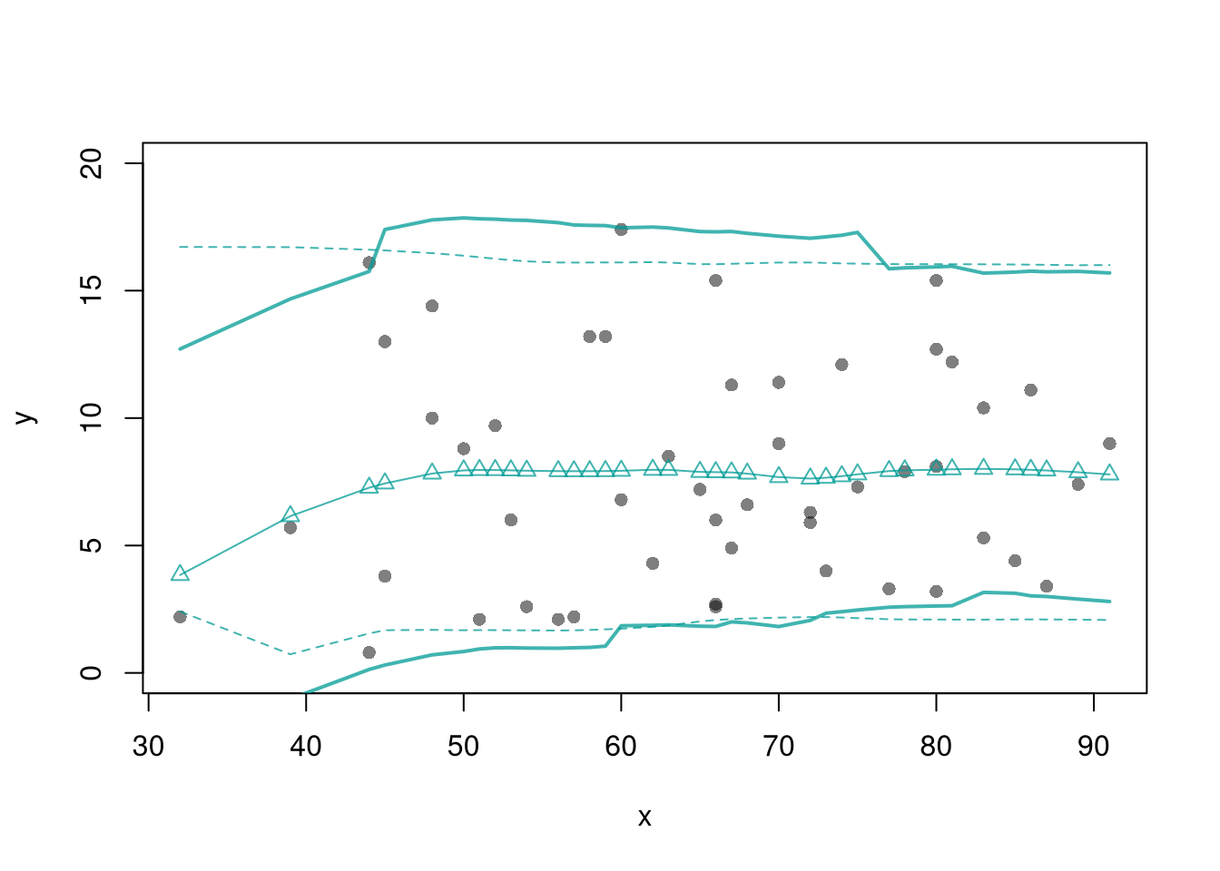

Code

# Bootstrap Prediction Interval
boot_resids <- lapply(boot_regs, function(reg_b){
    e_b <- resid(reg_b)
    x_b <- reg_b[['model']][['x']]
    res_b <- cbind(e_b, x_b)
})
boot_resids <- as.data.frame(do.call(rbind, boot_resids))
# Homoskedastic
ehat <- quantile(boot_resids[,'e_b'], probs=c(.025, .975))
x <- quantile(xy[,'x'],probs=seq(0,1,by=.1))
boot_pi <- coef(reg)[1] + x*coef(reg)['x']
boot_pi <- cbind(boot_pi + ehat[1], boot_pi + ehat[2])

# Plot Bootstrap PI
plot(y~x, dat=xy, pch=16, main='Prediction Intervals',
    ylim=c(-5,20), font.main=1)
polygon( c(x, rev(x)), c(boot_pi[,1], rev(boot_pi[,2])),
    col=grey(0,.2), border=NA)

# Parametric PI (For Comparison)
#pi <- predict(reg, interval='prediction', newdata=data.frame(x))
#lines( x, pi[,'lwr'], lty=2)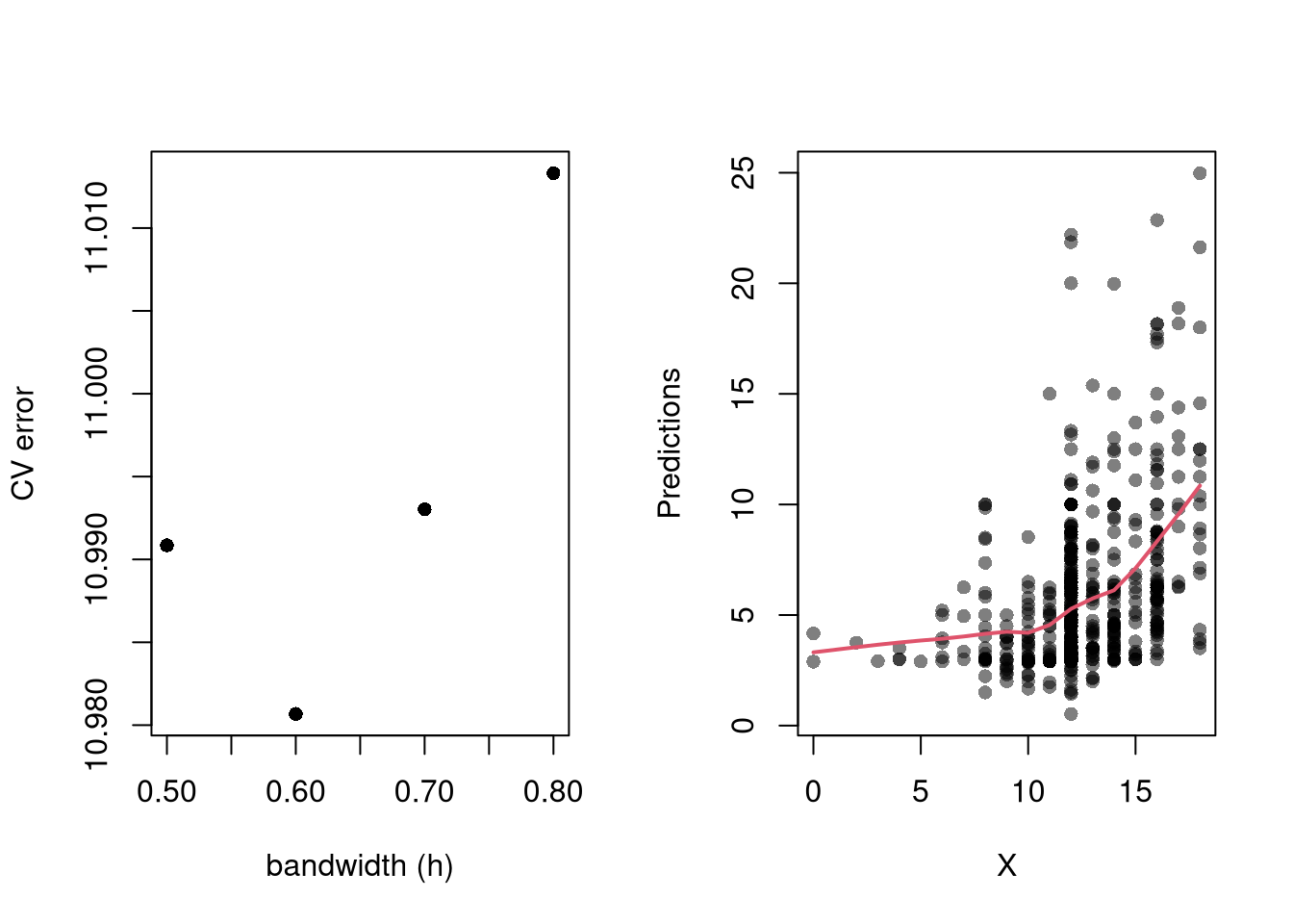
#lines( x, pi[,'upr'], lty=2)

Cross Validation.

Perhaps the most common approach to selecting a bandwidth is to minimize error. Leave-one-out Cross-validation minimizes the average “leave-one-out” mean square prediction errors: \[\begin{eqnarray} \min_{h} \quad \frac{1}{n} \sum_{i=1}^{n} \left[ \hat{Y}_{i} - \hat{y_{[i]}}(X,h) \right]^2, \end{eqnarray}\] where \(\hat{y}_{[i]}(X,h)\) is the model predicted value at \(X_{i}\) based on a dataset that excludes \(X_{i}\), and \(h\) is the bandwidth (e.g., bin size in a regressogram).

Minimizing out-sample prediction error is perhaps the simplest computational approach to choose bandwidths, and it also addresses an issue that plagues observational studies in the social sciences: your model explains everything and predicts nothing. Note, however, minimizing prediction error is not objectively “best”.

Code

library(wooldridge)
# Crossvalidated bandwidth for regression
xy_mat <- data.frame(x1=wage1[,'educ'],y=wage1[,'wage'])

## Grid Search
BWS <- c(0.5,0.6,0.7,0.8)
BWS_CV <- sapply(BWS, function(h){
    E_bw <- sapply(1:nrow(xy_mat), function(i){
        llls <- loess(y~x1, data=xy_mat[-i,], span=h, 
            degree=1, surface='direct')
        pred_i <- predict(llls, newdata=xy_mat[i,])
        e_i <-  (pred_i- xy_mat[i,'y'])
        return(e_i)
    })
    return( mean(E_bw^2) )
})

## Plot MSE
par(mfrow=c(1,2))
plot(BWS, BWS_CV, ylab='CV error', pch=16, 
    xlab='bandwidth (h)',)

## Plot Optimal Predictions
h_star <- BWS[which.min(BWS_CV)]
llls <- loess(y~x1, data=xy_mat, span=h_star, 
    degree=1, surface='direct')
plot(xy_mat, pch=16, col=grey(0,.5),
    xlab='X', ylab='Predictions')

pred_id <- order(xy_mat[,'x1'])
lines(xy_mat[pred_id,'x1'], predict(llls)[pred_id],
    col=2, lwd=2)

17.1 Objectives

Describe vs. Explain vs. Predict.

Prediction Intervals.

Cross Validation.

Bias vs. Variance