Just as with one sample tests, we can compute a standardized differences, where is converted into a statistic. Note, however, that we have to compute the standard error for the difference statistic, which is a bit more complicated. Under the assumption that both populations are independent distributed, we can analytically derive the sampling distribution for the differences between two groups.
In particular, the \(t\)-statistic is used to compare two groups. \[\begin{eqnarray}
\hat{t} = \frac{
\hat{M}_{Y1} - \hat{M}_{Y2}
}{
\sqrt{\hat{S}_{Y1}+\hat{S}_{Y2}}/\sqrt{n}
},
\end{eqnarray}\] With normally distributed means, this statistic follows Student’s t-distribution. Welch’s \(t\)-statistic is an adjustment for two normally distributed populations with potentially unequal variances or sample sizes. With the above assumptions, one can conduct hypothesis tests entirely using math.
Code
# Sample 1 (e.g., males)n1 <-100Y1 <-rnorm(n1, 0, 2)#hist(Y1, freq=F, main='Sample 1')# Sample 2 (e.g., females)n2 <-80Y2 <-rnorm(n2, 1, 1)#hist(Y2, freq=F, main='Sample 2')t.test(Y1, Y2, var.equal=F)## ## Welch Two Sample t-test## ## data: Y1 and Y2## t = -3.6628, df = 152.63, p-value = 0.0003435## alternative hypothesis: true difference in means is not equal to 0## 95 percent confidence interval:## -1.2692626 -0.3797979## sample estimates:## mean of x mean of y ## 0.2941225 1.1186527
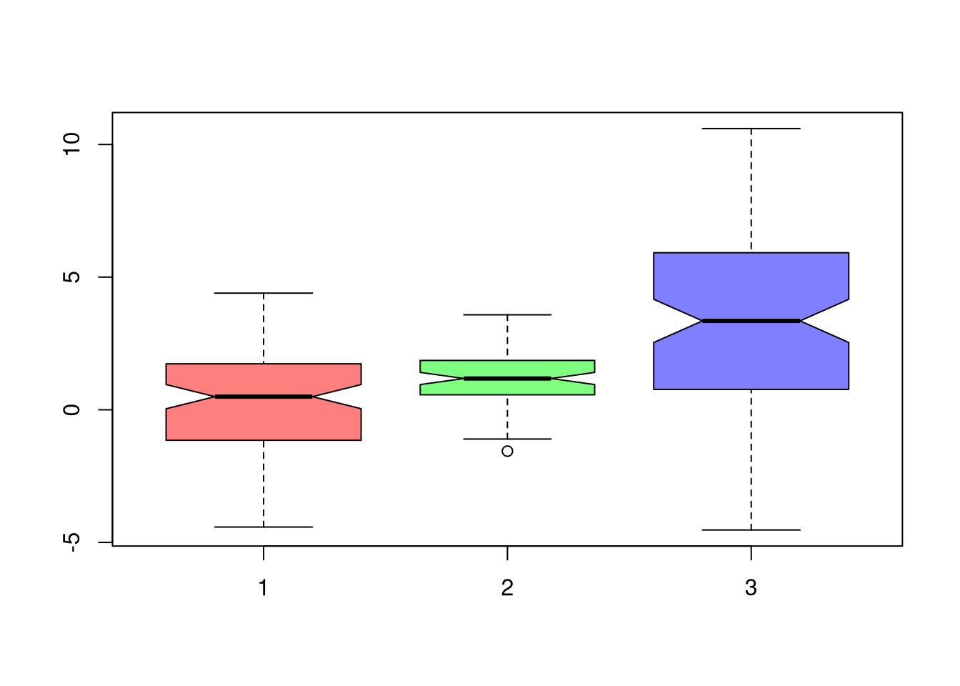
If we want to test for the differences in medians across groups with independent observations, we can also use notches in the boxplot. If the notches of two boxes do not overlap, then there is rough evidence that the difference in medians is statistically significant. The square root of the sample size is also shown as the bin width in each boxplot.1
When we test a hypothesis, we start with a claim called the null hypothesis \(H_0\) and an alternative claim \(H_A\). Because we base conclusions on sample data, which has variability, mistakes are possible. There are two types of errors:
Type I Error: Rejecting a true null hypothesis. (False Positive).
Type II Error: Failing to reject a false null hypothesis (False Negative).
True Situation
Decision: Fail to Reject \(H_0\)
Decision: Reject \(H_0\)
\(H_0\) is True
Correct (no detection)
Type I Error (False Positive)
\(H_0\) is False
Type II Error (False Negative; missed detection)
Correct (effect detected)
Tip
Here is a Courtroom example: Someone suspected of committing a crime is at trial, and they are either guilty or not (a Bernoulli random variable). You hypothesize that the suspect is innocent, and a jury can either convict them (decide guilty) or free them (decide not-guilty). Recall that fail-to-reject a hypothesis does mean accepting it, so deciding not-guilty does not necessarily mean innocent.
True Situation
Decision: Free
Decision: Convict
Suspect Innocent
Correctly Freed
Falsely Convicted
Suspect Guilty
Falsely Freed
Correctly Convicted
Statistical Power.
The probability of Type I Error is called significance level and denoted by \(Prob(\text{Type I Error}) = \alpha\). The probability of correctly rejecting a false null is called power and denoted by \(\text{Power} = 1 - \beta = 1 - Prob(\text{Type II Error})\).
Significance is often chosen by statistical analysts to be \(\alpha=0.05\). Power is less often chosen, instead following from a decision about power.
Tip
The code below runs a small simulation using a shifted, nonparametric bootstrap. Two-sided test; studentized statistic, for \(H0: \mu = 0\)
Code
# Power for Two-sided test;# nonparametric bootstrap, studentized statisticn <-25mu <-0alpha <-0.05B <-299sim_reps <-100p_values <-vector(length=sim_reps)for (i inseq(p_values)) {# Generate data X <-rnorm(n, mean=0.2, sd=1)# Observed statistic X_bar <-mean(X) T_obs <- (X_bar - mu) / (sd(X)/sqrt(n)) ##studentized# Bootstrap null distribution of the statistic T_boot <-vector(length=B) X_null <- X - X_bar + mu # Impose the null by recenteringfor (b inseq(T_boot)) { X_b <-sample(X_null, size = n, replace =TRUE) T_b <- (mean(X_b) - mu) / (sd(X_b)/sqrt(n)) T_boot[b] <- T_b }# Two-sided bootstrap p-value pval <-mean(abs(T_boot) >=abs(T_obs)) p_values[i] <- pval }power <-mean(p_values < alpha)power
There is an important Trade-off for fixed sample sizes: Increasing significance (fewer false positive) often lowers power (more false negatives). Generally, power depends on the effect size and sample size: bigger true effects and larger \(n\) make it easier to detect real differences (higher power, lower \(\beta\)).
Let each group \(g\) have median \(\tilde{M}_{g}\), interquartile range \(\hat{IQR}_{g}\), observations \(n_{g}\). We can compute standard deviation of the median as \(\tilde{S}_{g}= \frac{1.25 \hat{IQR}_{g}}{1.35 \sqrt{n_{g}}}\). As a rough guess, the interval \(\tilde{M}_{g} \pm 1.7 \tilde{S}_{g}\) is the historical default and displayed as a notch in the boxplot. See also https://www.tandfonline.com/doi/abs/10.1080/00031305.1978.10479236.↩︎