Code
# Simple random sample (no duplicates, equal probability)
x <- c(1, 2, 3, 4) # population
sample(x, 2, replace=F) #sample
## [1] 2 1A sample is a subset of the population. A simple random sample is a sample where each possible sample of size \(n\) has the same probability of being selected.
Often, we think of the population as being infinitely large. This is an approximation that makes mathematical and computational work much simpler.
#All possible samples of two from a bag of numbers {1, 2, 3, 4} with replacement
#{1, 1} {1, 2} {1, 3}, {3, 4}
#{2, 2} {2, 3} {2, 4}
#{3, 3} {3, 4}
#{4, 4}

# Simple random sample (duplicates, equal probability)
sample(x, 2, replace=T)
## [1] 3 2
Intuition for infinite populations: imagine drawing names from a giant urn. If the urn has only \(10\) names, then removing one name slightly changes the composition of the urn, and the probabilities shift for the next name you draw. Now imagine the urn has \(100\) billion names, so that removing one makes no noticeable difference. We can pretend the composition never changes: each draw is essentially identical and independent (iid). We can actually guarantee the names are iid by putting any names drawn back into the urn (sampling with replacement).
The sampling distribution of a statistic shows us how much a statistic varies from sample to sample.
For example, the sampling distribution of the mean shows how the sample mean varies from sample to sample to sample. The sampling distribution of mean can also be referred to as the probability distribution of the sample mean.
Given ages for population of \(4\) students, compute the sampling distribution for the mean with samples of \(n=2\).
X <- c(18, 20, 22, 24) # Ages for student population
# six possible samples
m1 <- mean( X[c(1, 2)] ) #{1, 2}
m2 <- mean( X[c(1, 3)] ) #{1, 3}
m3 <- mean( X[c(1, 4)] ) #{3, 4}
m4 <- mean( X[c(2, 3)] ) #{2, 3}
m5 <- mean( X[c(2, 4)] ) #{2, 4}
m6 <- mean( X[c(3, 4)] ) #{3, 4}
# sampling distribution
sample_means <- c(m1, m2, m3, m4, m5, m6)
hist(sample_means,
    freq=F, breaks=100,
    main=NA, border=NA)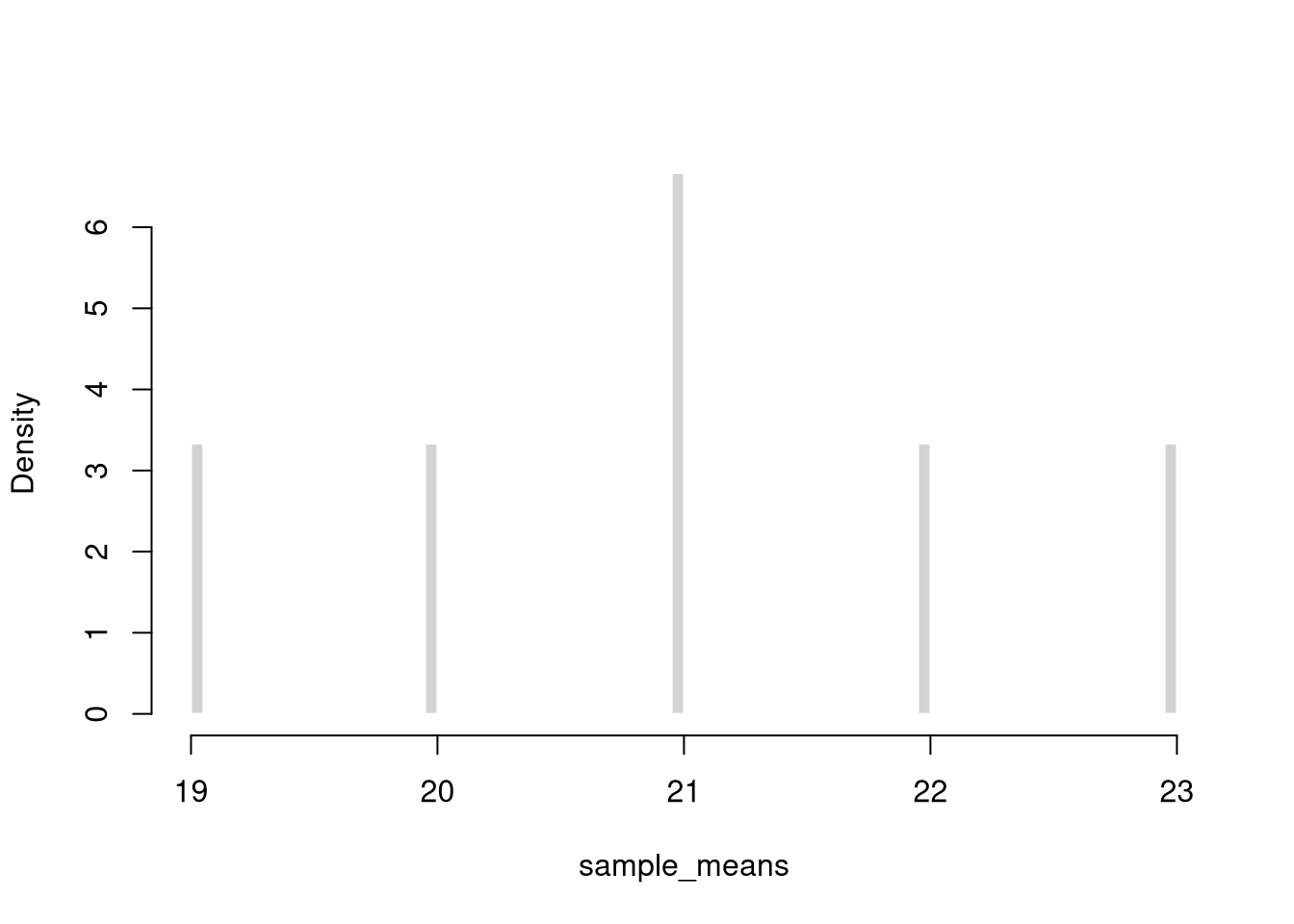
Now compute the sampling distribution for the median with samples of \(n=3\).
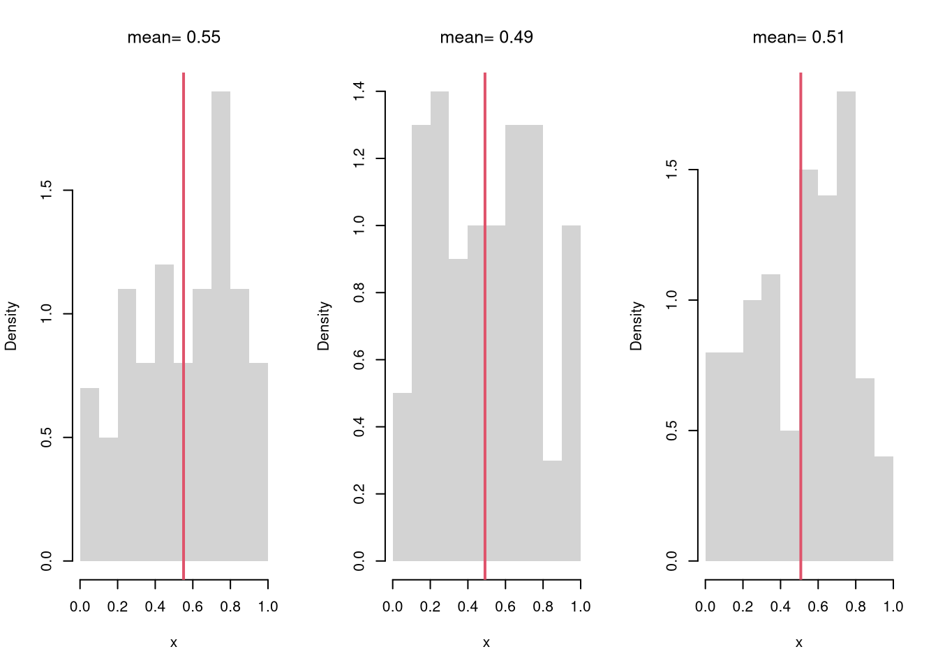
# Three Sample Example w/ Visual
par(mfrow=c(1, 3))
for(b in 1:3){
    x <- runif(100)
    m <-  mean(x)
    hist(x,
        breaks=seq(0, 1, by=.1), #for comparability
        freq=F, main=NA, border=NA)
    abline(v=m, col=rgb(1, 0, 0, .8), lwd=2)
    title(paste0('mean= ', round(m, 2)),  font.main=1)
}
Examine the sampling distribution of the mean
# Many sample example
sample_means <- rep(NA, 500)
for(i in seq_along(sample_means)){
    x <- runif(1000)
    m <- mean(x)
    sample_means[i] <- m
}
hist(sample_means,
    breaks=seq(0.45, 0.55, by=.001),
    border=NA, freq=F,
    col=rgb(1, 0, 0, .5),
    xlab=expression(hat(M)),
    main=NA)
title('Sampling Distribution of the mean', font.main=1)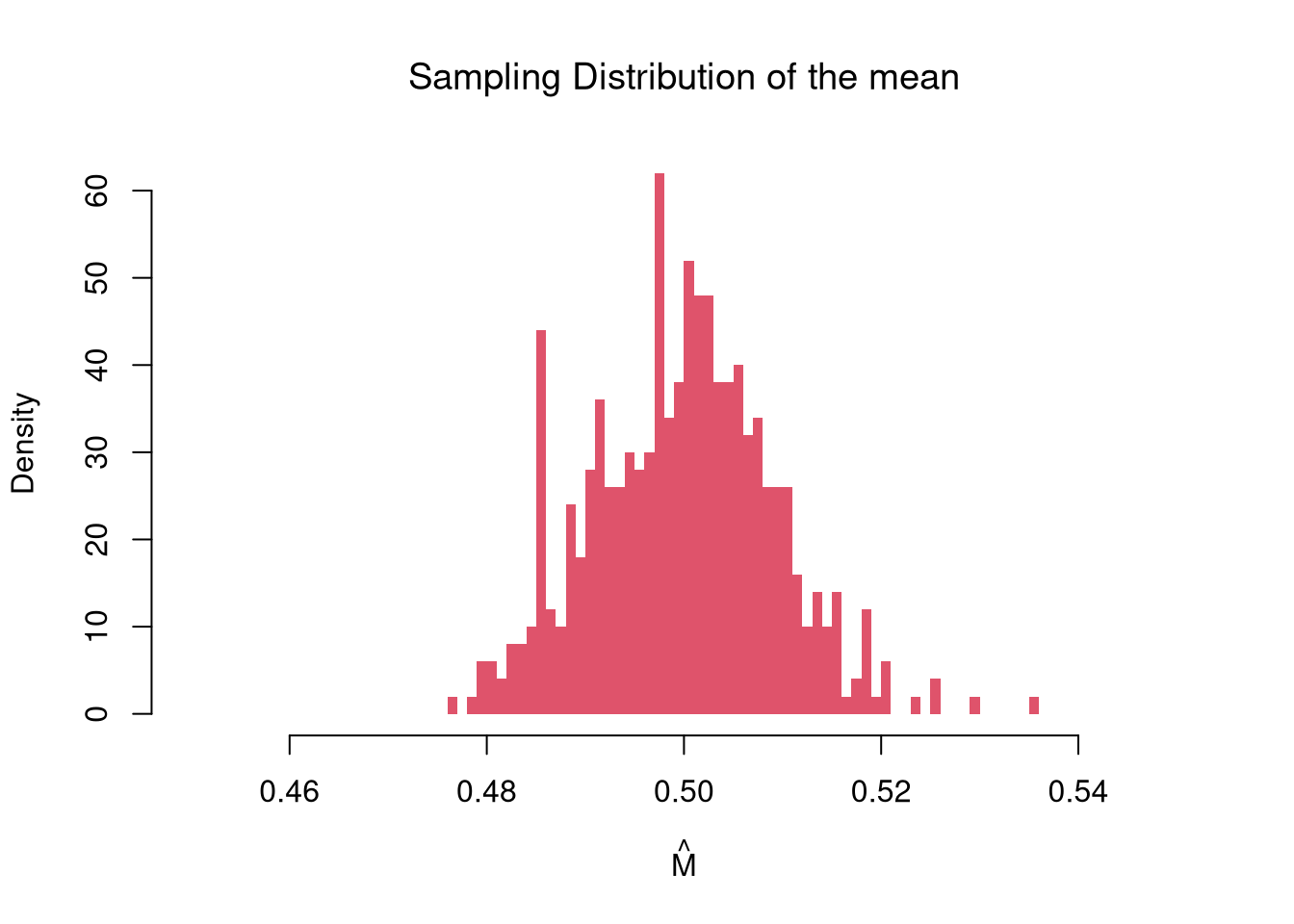
In this figure, you see two the most profound results known in statistics
There are different variants of the Law of Large Numbers (LLN), but they all say some version of “the sample mean becomes more tightly centered around the true mean as we get more data”.
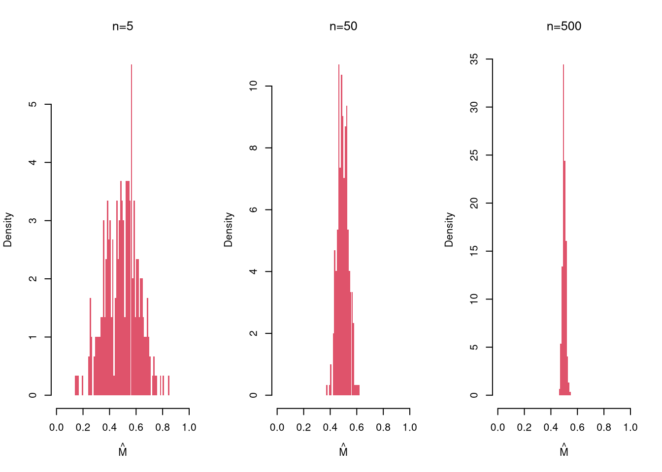
Notice where the sampling distribution is centered
m_LLLN <- mean(sample_means)
round(m_LLLN, 3)
## [1] 0.5
and more tightly centered with more data
par(mfrow=c(1, 3))
for(n in c(5, 50, 500)){
    sample_means_n <- rep(NA, 299)
    for(i in seq_along(sample_means_n)){
        x <- runif(n)
        m <- mean(x)
        sample_means_n[i] <- m
    }
    hist(sample_means_n,
        breaks=seq(0, 1, by=.01),
        border=NA, freq=F,
        col=rgb(1, 0, 0, .5),
        xlab=expression(hat(M)),
        main=NA)
    title(paste0('n=', n), font.main=1)
}
Plot the variability of the sample mean as a function of sample size
n_seq <- seq(1, 40)
sd_seq <- rep(NA, length(n_seq))
for(n in seq_along(sd_seq)){
    sample_means_n <- rep(NA, 499)
    for(i in seq_along(sample_means_n)){
        x <- runif(n)
        m <- mean(x)
        sample_means_n[i] <- m
    }
    sd_seq[n] <- sd(sample_means_n)
}
plot(n_seq, sd_seq, pch=16, col=grey(0, 0.5),
    xlab='n', ylab='sd of sample means', main=NA)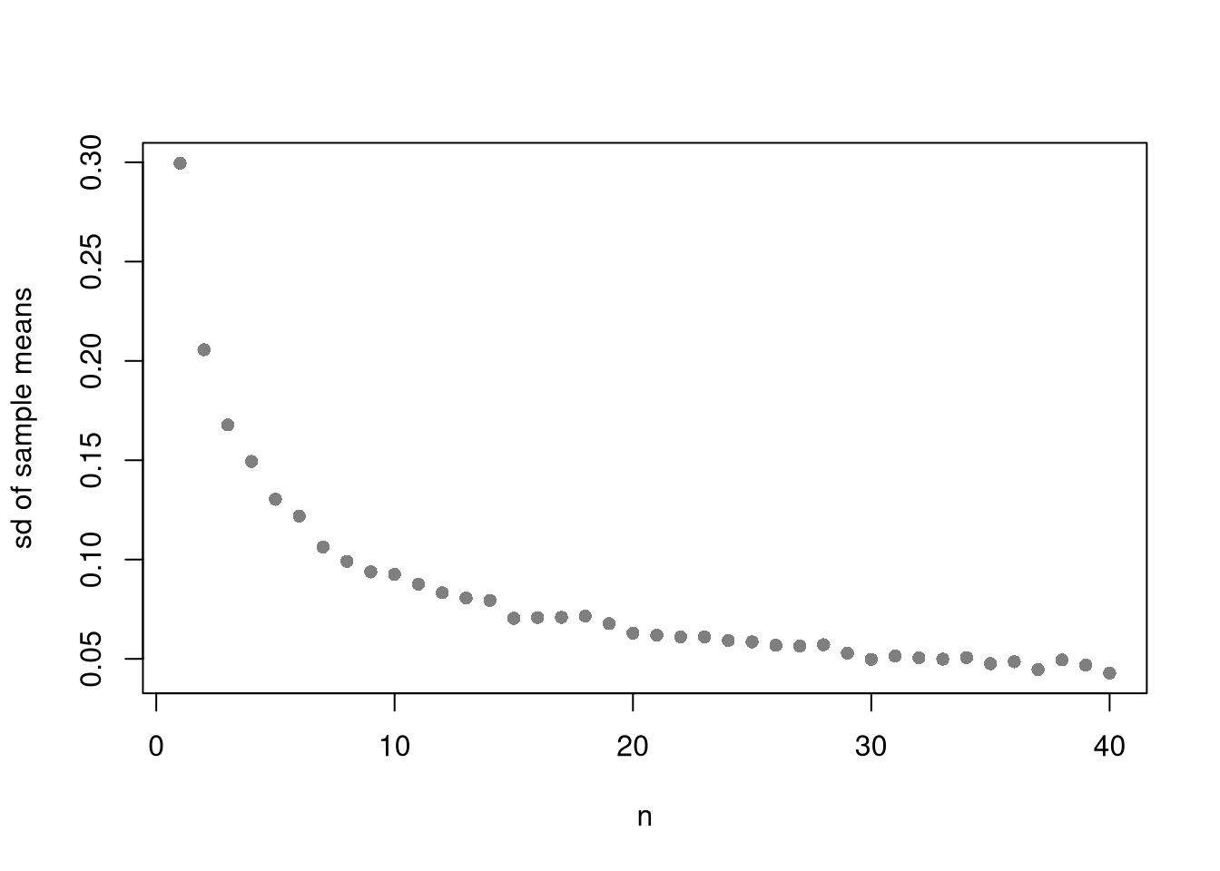
Here is the intuition for estimating the mean weight of an apple:
There are different variants of the central limit theorem (CLT), but they all say some version of “the sampling distribution of the mean is approximately normal”. For example, the sampling distribution of the mean, shown above, is approximately normal.
hist(sample_means,
    breaks=seq(0.45, 0.55, by=.001),
    border=NA, freq=F,
    col=rgb(1, 0, 0, .5),
    xlab=expression(hat(M)),
    main=NA)
title('Sampling Distribution of the mean', font.main=1)

# Approximately normal?
mu <- mean(sample_means)
mu_sd <- sd(sample_means)
x <- seq(0.1, 0.9, by=0.001)
fx <- dnorm(x, mu, mu_sd)
lines(x, fx, col=rgb(1, 0, 0, .8))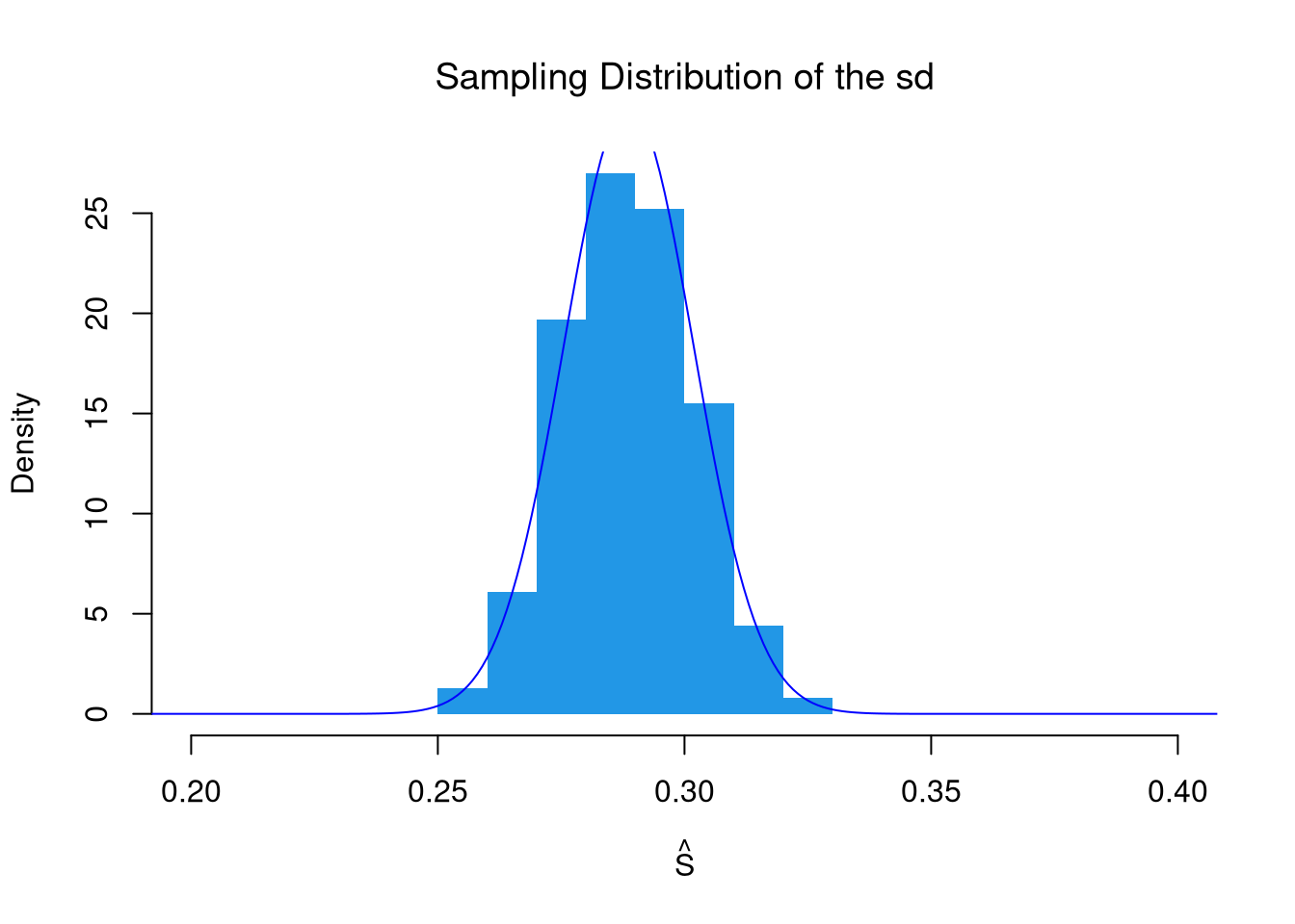
Many statistics have an approximately Normal sampling distribution.
For an example with another statistic, let’s the sampling distribution of the standard deviation.
# CLT example of the 'sd' statistic
sample_sds <- rep(NA, 1000)
for(i in seq_along(sample_sds)){
    x <- runif(100) # same distribution
    s <- sd(x) # different statistic
    sample_sds[i] <- s
}
hist(sample_sds,
    breaks=seq(0.2, 0.4, by=.01),
    border=NA, freq=F,
    col=rgb(0, 0, 1, .5),
    xlab=expression(hat(S)),
    main=NA)
title('Sampling Distribution of the sd', font.main=1)

# Approximately normal?
mu <- mean(sample_sds)
mu_sd <- sd(sample_sds)
x <- seq(0.1, 0.9, by=0.001)
fx <- dnorm(x, mu, mu_sd)
lines(x, fx, col=rgb(0, 0, 1, .8))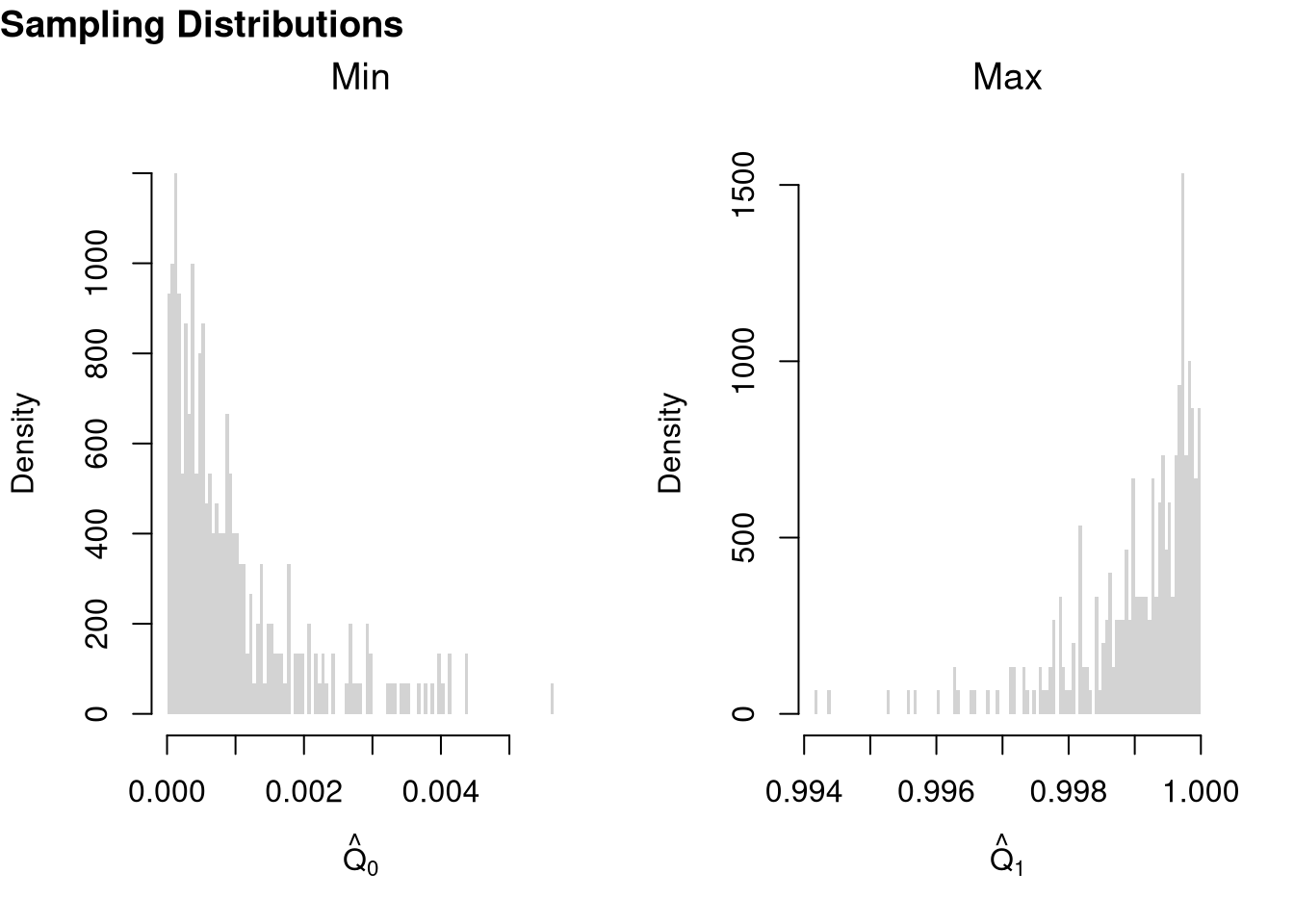
# try another random variable, such as rexp(100) instead of runif(100)It is beyond this class to prove this result mathematically, but you should know that not all sampling distributions are standard normal. The CLT approximation is better for “large \(n\)” datasets with “well behaved” variances. The CLT also does not apply to “extreme” statistics.
For example of “extreme” statistics, examine the sampling distribution of min and max statistics.
# Create 300 samples, each with 1000 random uniform variables
x_samples <- matrix(nrow=300, ncol=1000)
for(i in seq(1, nrow(x_samples))){
    x_samples[i, ] <- runif(1000)
}
# Each row is a new sample
length(x_samples[1, ])
## [1] 1000

# Compute min and max for each sample
x_mins <- apply(x_samples, 1, quantile, probs=0)
x_maxs <- apply(x_samples, 1, quantile, probs=1)

# Plot the sampling distributions of min, median, and max
# Median looks normal. Maximum and minimum do not!
par(mfrow=c(1, 2))
hist(x_mins, breaks=100, main=NA,
    xlab=expression(hat(Q)[0]), border=NA, freq=F)
title('Min', font.main=1)
hist(x_maxs, breaks=100, main=NA,
    xlab=expression(hat(Q)[1]), border=NA, freq=F)
title('Max', font.main=1)
title('Sampling Distributions', outer=T, line=-1, adj=0, font.main=1)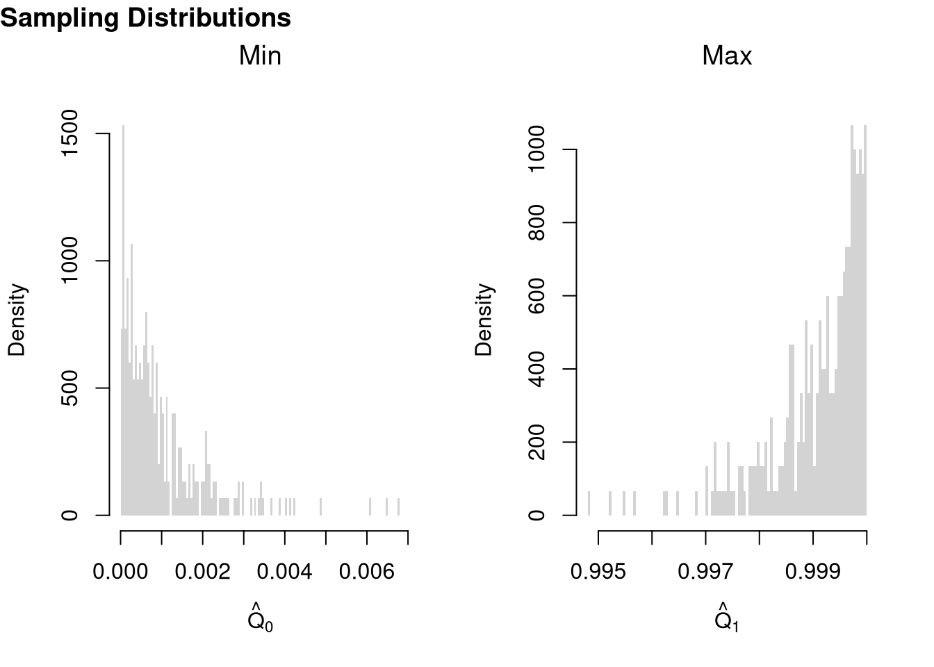
Explore another function, such as my_function <- function(x){ diff(range(x)) }
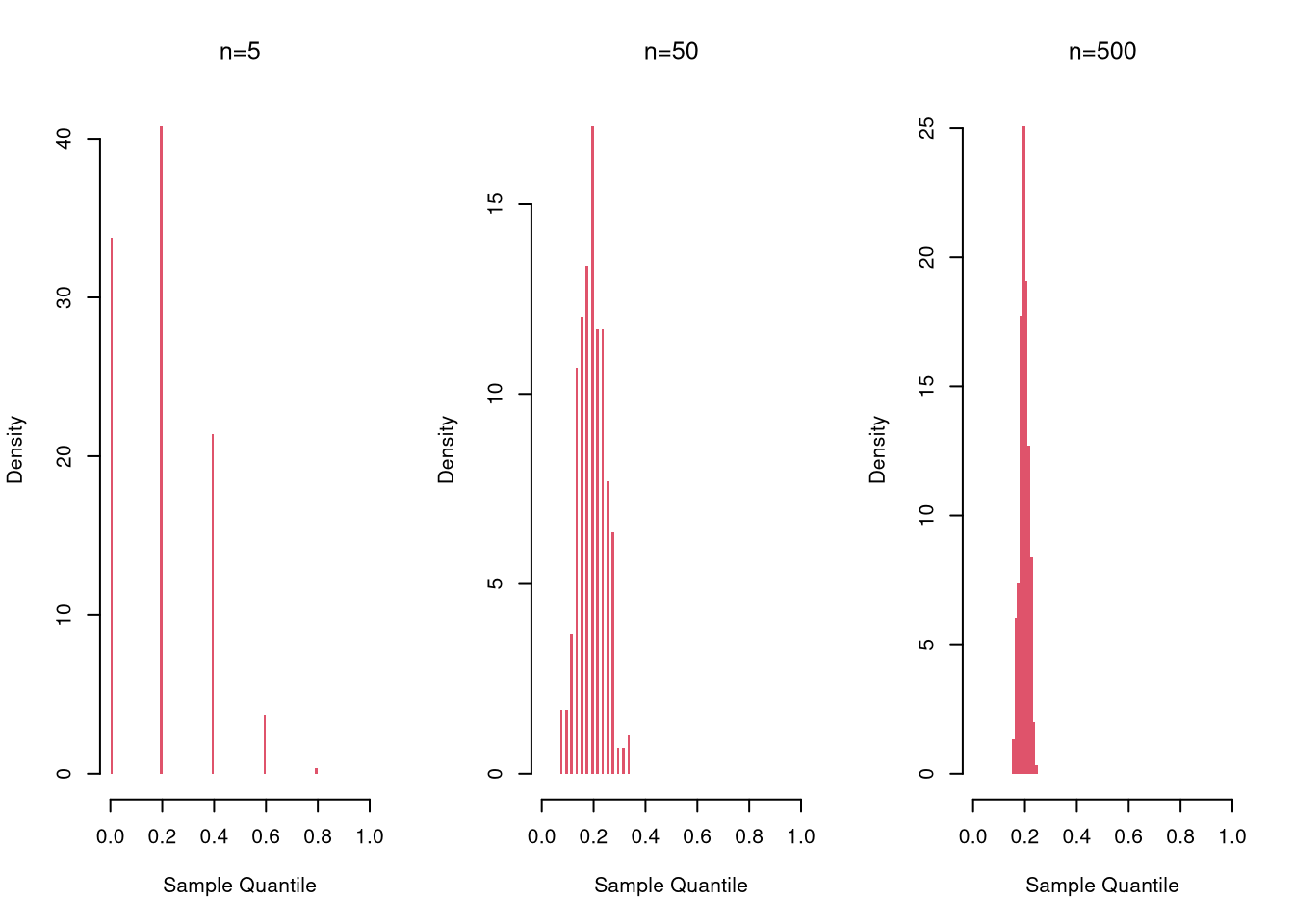
The Law of Large Numbers generalizes to many other statistics, like median or sd.1
Here is a sampling distribution for a quantile, for three different sample sizes
par(mfrow=c(1, 3))
for(n in c(5, 50, 500)){
    sample_quants_n <- rep(NA, 299)
    for(i in seq_along(sample_quants_n)){
        x <- runif(n)
        m <- quantile(x, probs=0.75) #upper quartile
        sample_quants_n[i] <- m
    }
    hist(sample_quants_n,
        breaks=seq(0, 1, by=.01),
        border=NA, freq=F,
        col=rgb(1, 0, 0, .5),
        xlab='Sample Quantile',
        main=NA)
    title(paste0('n=', n), font.main=1)
}
Here is a sampling distribution for a proportion, for three different sample sizes
par(mfrow=c(1, 3))
for(n in c(5, 50, 500)){
    sample_props_n <- rep(NA, 299)
    for(i in seq_along(sample_props_n)){
        x <- sample(1:5, size=n, prob=c(1:5)/15, replace=T)
        p3 <- mean(x==3)
        sample_props_n[i] <- p3
    }
    hist(sample_props_n,
        breaks=seq(0, 1, by=.01),
        border=NA, freq=F,
        col=rgb(1, 0, 0, .5),
        xlab='Sample Proportion',
        main=NA)
    title(paste0('n=', n), font.main=1)
}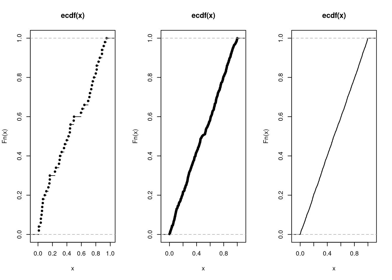
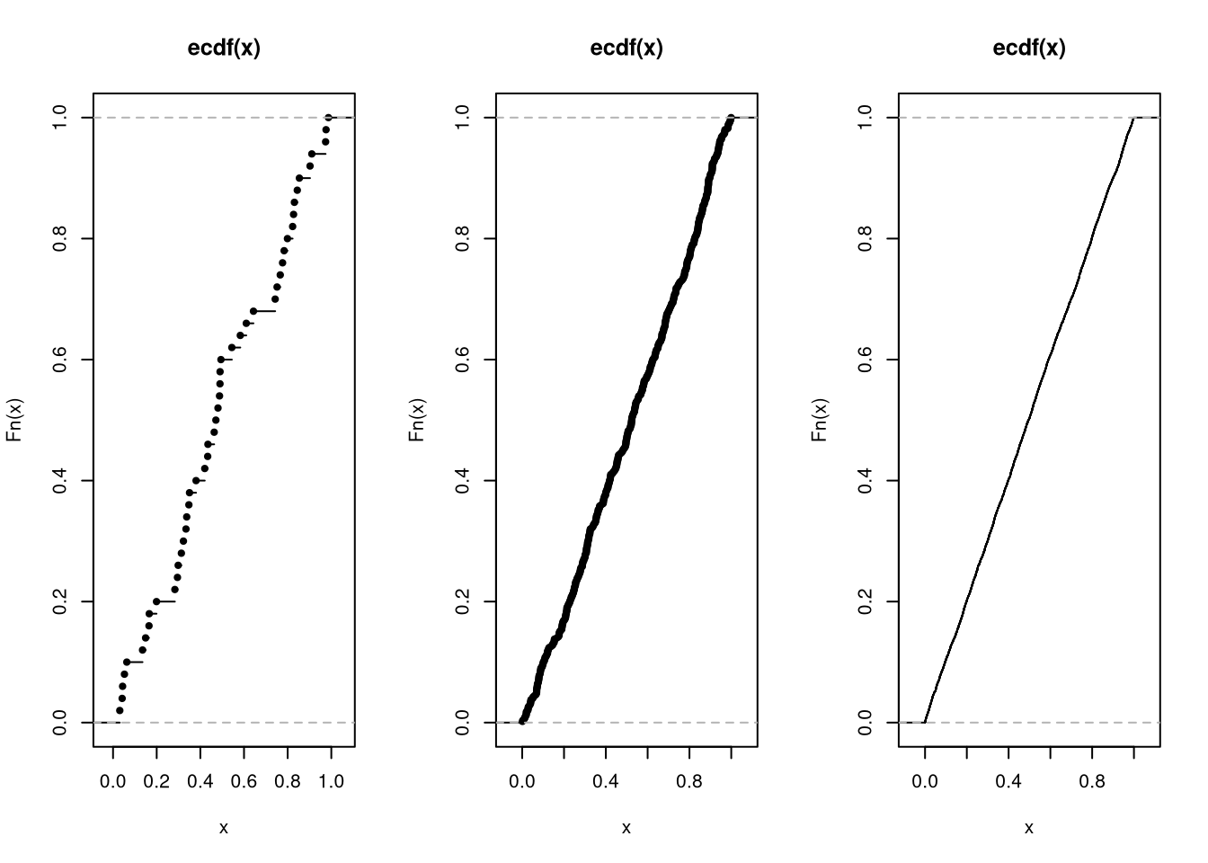
In fact, the Glivenko-Cantelli Theorem (GCT) shows entire empirical distribution converges: the ECDF gets increasingly close to the CDF as the sample sizes grow. This result is often termed the The Fundamental Theorem of Statistics.
par(mfrow = c(1, 3))
for (n in c(50, 500, 5000)) {
  x <- runif(n)
  Fx <- ecdf(x)
  plot(Fx, main=NA)
  title(paste0('n=', n), font.main=1)
}
Often, we only have one sample. How then can we estimate the sampling distribution of a statistic?
sample_dat <- USArrests[, 'Murder']
sample_mean <- mean(sample_dat)
sample_mean
## [1] 7.788
We can resample our data. Hesterberg (2015) provides a nice illustration of the idea. The two most basic versions are the jackknife and the bootstrap, which are discussed below.
Note that we do not use the mean of the resampled statistics as a replacement for the original estimate. This is because the resampled distributions are centered at the observed statistic, not the population parameter. (The bootstrapped mean is centered at the sample mean, for example, not the population mean.) This means that we do not use resampling to improve on \(\hat{M}\). We use resampling to estimate sampling variability.
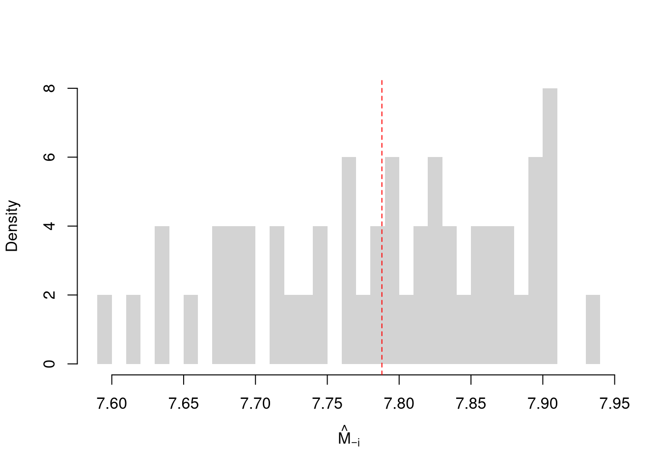
Here, we compute all “leave-one-out” estimates. Specifically, for a dataset with \(n\) observations, the jackknife uses \(n-1\) observations other than \(i\) for each unique subsample.
sample_dat <- USArrests[, 'Murder']
sample_mean <- mean(sample_dat)

# Jackknife Estimates
n <- length(sample_dat)
jackknife_means <- rep(NA, n)
for(i in seq_along(jackknife_means)){
    dat_noti <- sample_dat[-i]
    mean_noti <- mean(dat_noti)
    jackknife_means[i] <- mean_noti
}
hist(jackknife_means, breaks=25,
    border=NA, freq=F,
    main=NA, xlab=expression(hat(M)[-i]))
abline(v=sample_mean, col=rgb(1, 0, 0, .8), lty=2)
Here, we draw \(n\) observations with replacement from the original data to create a bootstrap sample and calculate a statistic. Each bootstrap sample \(b=1...B\) uses a random resample of the observations to recompute a statistic. We repeat that many times, say \(B=9999\), to estimate the sampling distribution.
# Bootstrap estimates
bootstrap_means <- rep(NA, 9999)
for(b in seq_along(bootstrap_means)){
    boot_id <- sample(n, replace=T)
    dat_b  <- sample_dat[boot_id] # c.f. jackknife
    mean_b <- mean(dat_b)
    bootstrap_means[b] <-mean_b
}

hist(bootstrap_means, breaks=25,
    border=NA, freq=F,
    main=NA, xlab=expression(hat(M)[b]))
abline(v=sample_mean, col=rgb(1, 0, 0, .8), lty=2)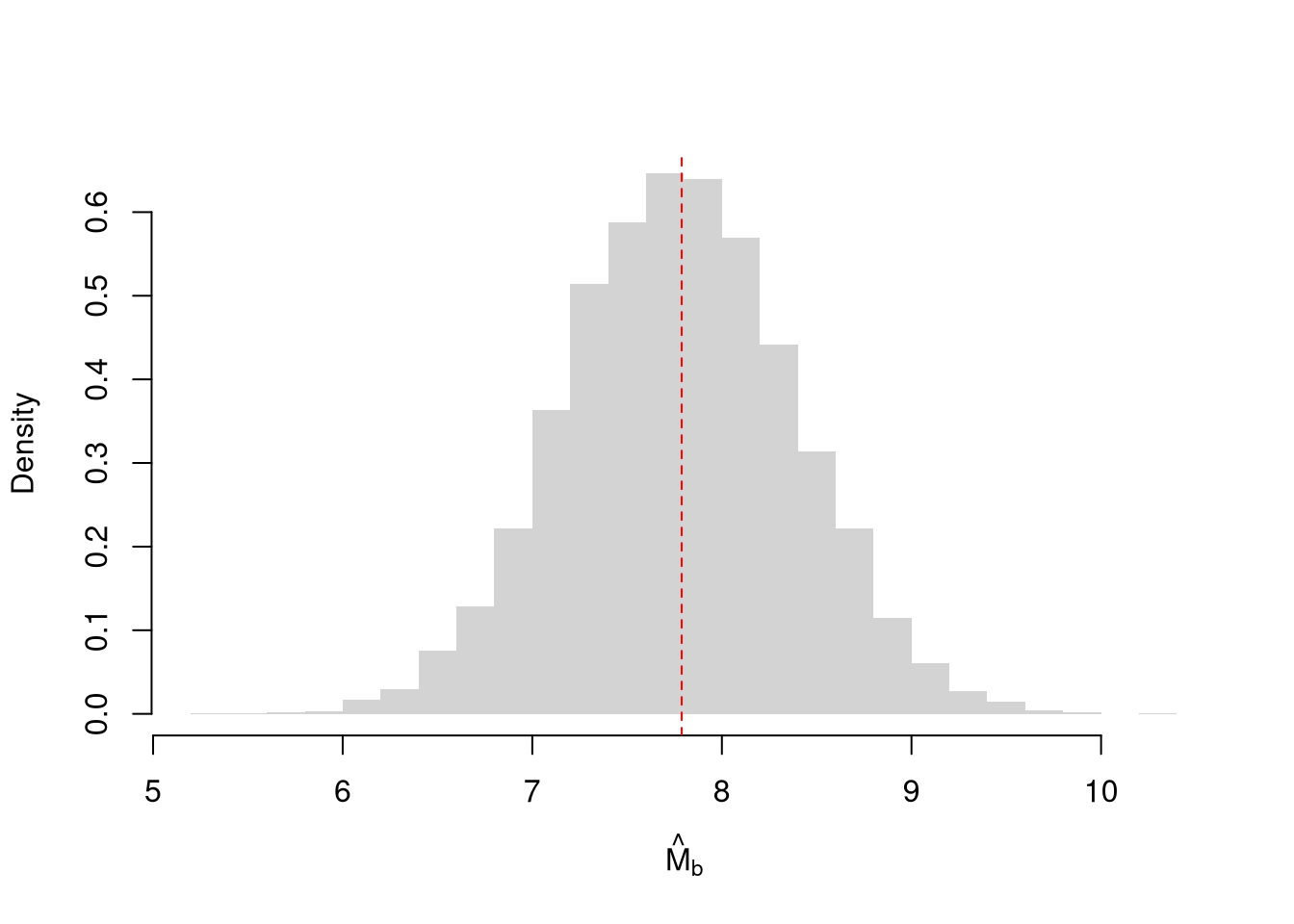
Why does this work? The sample: \(\{\hat{X}_{1}, \hat{X}_{2}, ... \hat{X}_{n}\}\) is drawn from a CDF \(F\). Each bootstrap sample: \(\{\hat{X}_{1}^{(b)}, \hat{X}_{2}^{(b)}, ... \hat{X}_{n}^{(b)}\}\) is drawn from the ECDF \(\hat{F}\). With \(\hat{F} \approx F\), each bootstrap sample is approximately a random sample. So when we compute a statistic on each bootstrap sample, we approximate the sampling distribution of the statistic.
Note that both Jackknife and Bootstrap resampling methods provide imperfect estimates, and can give different numbers.
Using either the bootstrap or jackknife distribution, we typically communicate the variability of the sampling distribution of a statistic using the Standard Error. In either case, this differs from the standard deviation of the data within your sample.
For a bootstrap example
Also note that each additional data point you have provides more information, which ultimately decreases the standard error of your estimates. This is why statisticians will often recommend that you to get more data. However, the improvement in the standard error increases at a diminishing rate. In economics, this is known as diminishing returns and why economists may recommend you do not get more data.
B <- 999 # number of bootstrap samples
Nseq <- seq(1, length(sample_dat), by=1) # different resample sizes
n_id <- seq_along(sample_dat) # who to potentially resample

## For each sample size, compute the bootstrap SE
SE <- rep(NA, length(Nseq))
for(n in seq_along(Nseq)){
    sample_stats_n <- rep(NA, B)
    for(b in seq(1, B)){
        b_id <- sample(n_id, size=n, replace=T)
        x_b <- sample_dat[b_id]
        x_stat_b <- mean(x_b) # statistic of interest
        sample_stats_n[b] <- x_stat_b
    }
    se_n <- sd(sample_stats_n) # How much the statistic varies across samples
    SE[n] <- se_n
}

plot(Nseq, SE, pch=16, col=grey(0, 0.5),
    ylab='standard error', xlab='sample size', main=NA)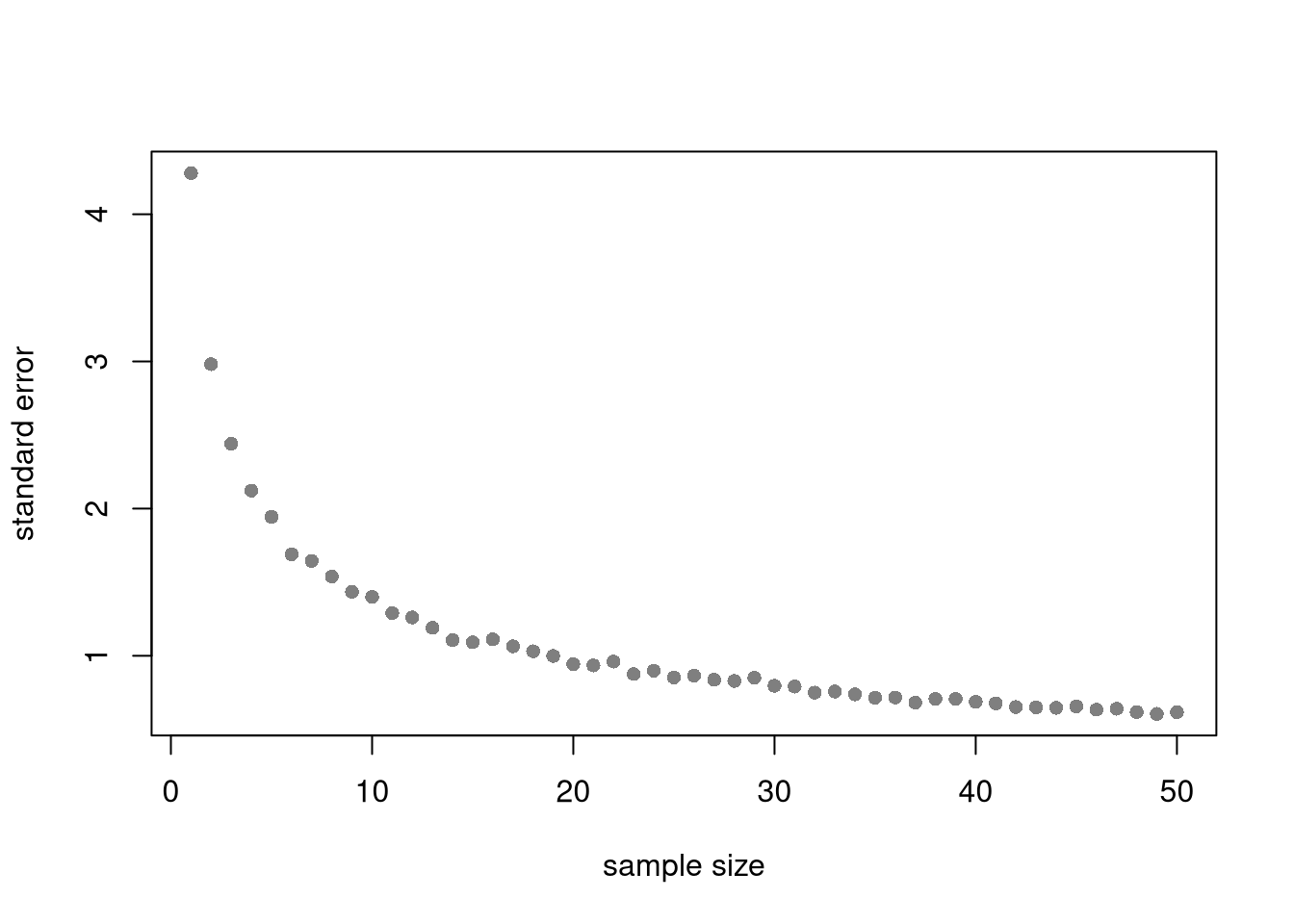
The above procedure works for many different statistics
med <- quantile(sample_dat, prob=0.5)

# Bootstrap estimates
bootstrap_stat <- rep(NA, 9999)
for(b in seq_along(bootstrap_stat)){
    boot_id <- sample(n, replace=T)
    dat_b  <- sample_dat[boot_id] # c.f. jackknife
    stat_b <- quantile(dat_b, prob=0.5)
    bootstrap_stat[b] <- stat_b
}

hist(bootstrap_stat, breaks=25,
    border=NA, freq=F,
    main=NA, xlab=expression(Med[b]))
abline(v=med, col=rgb(1, 0, 0, .8), lty=2)
This means we can compute bootstrap SEs for other statistics, too.
To generate a random variable from known distributions, you can use some type of physical machine. E.g., you can roll a fair die to generate Discrete Uniform data or you can roll weighted die to generate Categorical data.
There are also several ways to computationally generate random variables from a probability distribution. Perhaps the most common one is inverse sampling. To generate a random variable using inverse sampling, first sample \(p\) from a uniform distribution and then find the associated quantile quantile function \(\hat{F}^{-1}(p)\).2
You can generate a random variable from a known empirical distribution. Inverse sampling randomly selects observations from the dataset with equal probabilities. To implement this, we
Here is an example of generating random murder rates for US states.
# Empirical Distribution
X <- USArrests[, 'Murder']
FX_hat <- ecdf(X)
plot(FX_hat, lwd=2, xlim=c(0, 20),
    pch=16, col=grey(0, .5), main=NA)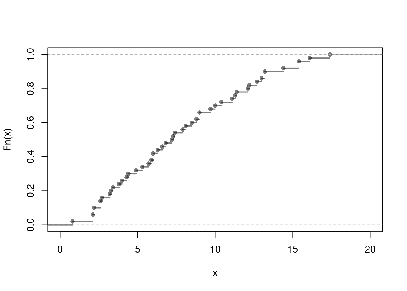
# Generating random variables via inverse ECDF
p <- runif(3000) ## Multiple Draws
QX_hat <- quantile(FX_hat, p, type=1)
QX_hat[c(1, 2, 3)]
## 67.03324958% 22.58107369%  8.96678311%
##          9.7          3.8          2.2

## Can also do directly from the data
QX_hat <- quantile(X, p, type=1)
QX_hat[c(1, 2, 3)]
## 67.03324958% 22.58107369%  8.96678311%
## 9.7 3.8 2.2If you know the distribution function that generates the data, then you can derive the quantile function and do inverse sampling. That is how computers generate random data from a distribution.
# 4 random data points from 3 different distributions
qunif(4)
## [1] NaN
qexp(4)
## [1] NaN
qnorm(4)
## [1] NaN
Here is an in-depth example of the Dagum distribution. The distribution function is \(F(x)=(1+(x/b)^{-a})^{-c}\). For a given probability \(p\), we can then solve for the quantile as \(F^{-1}(p)=\frac{ b p^{\frac{1}{ac}} }{(1-p^{1/c})^{1/a}}\). Afterwhich, we sample \(p\) from a uniform distribution and then find the associated quantile.
# Theoretical Quantile Function (from VGAM::qdagum)
qdagum <- function(p, scale.b=1, shape1.a, shape2.c) {
  # Quantile function (theoretically derived from the CDF)
  ans <- scale.b * (expm1(-log(p) / shape2.c))^(-1 / shape1.a)
  # Special known cases
  ans[p == 0] <- 0
  ans[p == 1] <- Inf
  # Safety Checks
  ans[p < 0] <- NaN
  ans[p > 1] <- NaN
  if(scale.b <= 0 | shape1.a <= 0 | shape2.c <= 0){ ans <- ans*NaN }
  # Return
  return(ans)
}

# Generate Random Variables (VGAM::rdagum)
rdagum <-function(n, scale.b=1, shape1.a, shape2.c){
    p <- runif(n) # generate random probabilities
    x <- qdagum(p, scale.b=scale.b, shape1.a=shape1.a, shape2.c=shape2.c) #find the inverses
    return(x)
}

# Example
set.seed(123)
X <- rdagum(3000, 1, 3, 1)
X[c(1, 2, 3)]
## [1] 0.7390476 1.5499868 0.8845006In your own words, explain the difference between the standard deviation of a sample and the standard error of the sample mean. Why does the standard error decrease as \(n\) grows, while the standard deviation does not necessarily change?
Consider a population of four students with ages \(\{18, 20, 22, 24\}\). List all possible simple random samples of size \(n=2\) (without replacement). Compute the sample mean for each. Then compute the mean and standard deviation of those sample means. Verify that the mean of the sample means equals the population mean.
Load USArrests in R and extract the UrbanPop column. Write a bootstrap loop with \(B=5000\) resamples to estimate the standard error of the median. That is, for each resample draw n observations with replacement, compute the median, store it, and then compute sd of the stored medians. Compare this bootstrap standard error to the bootstrap standard error of the mean from the same data.