Just as with one sample tests, we can compute standardized differences. The observed difference is converted into a \(t\)-statistic by dividing by an estimated standard error. Note, however, that we have to compute the standard error for the difference statistic, which is a bit more complicated than for a single sample. Under the assumption that both populations are independently distributed, we can analytically derive the sampling distribution for the differences between two groups.
Differences in Means.
In particular, the \(t\)-statistic is used to compare two groups. \[\begin{eqnarray}
\hat{t} = \frac{
\hat{M}_{Y1} - \hat{M}_{Y2}
}{
\sqrt{\hat{S}^2_{Y1}/n_1+\hat{S}^2_{Y2}/n_2}
},
\end{eqnarray}\] where \(\hat{S}^2_{Yg}\) is the sample variance and \(n_g\) is the sample size for group \(g\). With normally distributed means, this statistic follows Student’s t-distribution. Welch’s \(t\)-statistic is an adjustment for two normally distributed populations with potentially unequal variances or sample sizes. The degrees of freedom are approximated by the Welch-Satterthwaite equation. With the above assumptions, one can conduct hypothesis tests entirely using math.
Code
# Sample 1 (e.g., males)n1 <-100Y1 <-rnorm(n1, 0, 2)#hist(Y1, freq=F, main='Sample 1')# Sample 2 (e.g., females)n2 <-80Y2 <-rnorm(n2, 1, 1)#hist(Y2, freq=F, main='Sample 2')t.test(Y1, Y2, var.equal=F)## ## Welch Two Sample t-test## ## data: Y1 and Y2## t = -5.9446, df = 154.8, p-value = 1.773e-08## alternative hypothesis: true difference in means is not equal to 0## 95 percent confidence interval:## -1.6144064 -0.8090767## sample estimates:## mean of x mean of y ## -0.05741869 1.15432285
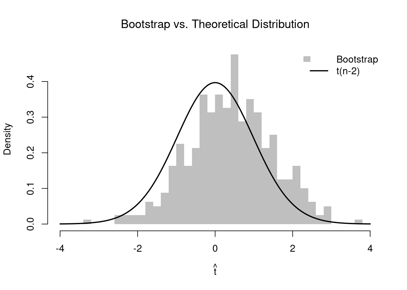
We can visualize this by simulating many samples under the null (\(\mu_1=\mu_2\)) and comparing the distribution of \(\hat{t}\) with the theoretical \(t\)-distribution.
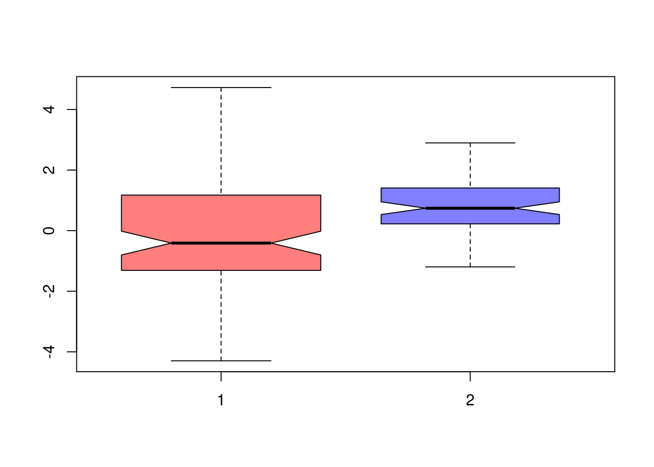
If we want to test for the differences in medians across groups with independent observations, we can also use notches in the boxplot. If the notches of two boxes do not overlap, then there is rough evidence that the difference in medians is statistically significant. The square root of the sample size is also shown as the bin width in each boxplot.1
There are also non-parametric alternatives for distributional comparisons. The Mann-Whitney U test compares distributions using ranks rather than assuming normality.
The same ideas apply to regression coefficients. Recall that the OLS slope \(\hat{b}_1 = \hat{C}_{XY}/\hat{V}_X\) is a statistic computed from the data. In the Simple Regression chapter, we estimated variability using data-driven methods (jackknife and bootstrap). Under standard assumptions, we can instead derive the sampling distribution analytically: the \(t\)-statistic \[\begin{eqnarray}
\hat{t} = \frac{\hat{b}_1}{\hat{s}_{\hat{b}_1}}
\end{eqnarray}\] follows a \(t\)-distribution with \(n-2\) degrees of freedom, where \(\hat{s}_{\hat{b}_1}\) is the standard error of the slope. This allows us to test \(H_0: \beta_1 = 0\) using math alone.
Code
# USArrests data (same as Simple Regression chapter)xy <- USArrests[, c('Murder', 'UrbanPop')]colnames(xy) <-c('y', 'x')reg <-lm(y ~ x, data = xy)# The summary reports theoretical t-statistics and p-valuessummary(reg)$coefficients## Estimate Std. Error t value Pr(>|t|)## (Intercept) 6.41594246 2.90669257 2.2073000 0.03210725## x 0.02093466 0.04332647 0.4831841 0.63116178
NoteMust Know
Manual verification of the theoretical \(t\)-statistic for the slope:
Code
n <-nrow(xy)b1 <-coef(reg)[2]e <-resid(reg)s_e <-sqrt(sum(e^2) / (n -2)) # residual standard errors_b1 <- s_e /sqrt(sum((xy[, 'x'] -mean(xy[, 'x']))^2)) # SE of slopet_stat <- b1 / s_b1# Compare with summary outputc(manual = t_stat, summary =summary(reg)$coefficients[2, 3])## manual.x summary ## 0.4831841 0.4831841
We can compare the bootstrap sampling distribution of \(\hat{t}\) (histogram) with the theoretical \(t_{n-2}\) distribution (curve). They should be similar, but are not identical because the theoretical result assumes normally distributed errors.
Code
# Bootstrap distribution of the t-statisticn <-nrow(xy)B <-399boot_t <-vector(length = B)for (b inseq(B)) { b_id <-sample(nrow(xy), replace =TRUE) xy_b <- xy[b_id, ] reg_b <-lm(y ~ x, data = xy_b)# Use theoretical SE from summary boot_t[b] <-summary(reg_b)$coefficients[2, 3]}# Overlay: bootstrap histogram vs. theoretical t-distributiont_range <-range(c(boot_t, -4, 4))hist(boot_t, breaks =30, freq =FALSE, border =NA,col =grey(0.5, 0.5),xlim = t_range,xlab =expression(hat(t)),main =NA)title('Bootstrap vs. Theoretical Distribution', font.main =1)# Theoretical t(n-2) densityt_grid <-seq(t_range[1], t_range[2], length =200)lines(t_grid, dt(t_grid, df = n -2), lwd =2)legend('topright', legend =c('Bootstrap', 't(n-2)'),fill =c(grey(0.5, 0.5), NA), border =NA,lwd =c(NA, 2), lty =c(NA, 1), bty ='n')
We can compute the \(p\)-value for \(H_0: \beta_1 = 0\) two ways: from the theoretical \(t\)-distribution and from the bootstrap distribution. Both ask how extreme the observed \(\hat{t}\) is under the null.
When we test a hypothesis, we start with a claim called the null hypothesis \(H_0\) and an alternative claim \(H_A\). Because we base conclusions on sample data, which has variability, mistakes are possible. There are two types of errors:
Type I Error: Rejecting a true null hypothesis. (False Positive).
Type II Error: Failing to reject a false null hypothesis (False Negative).
True Situation
Decision: Fail to Reject \(H_0\)
Decision: Reject \(H_0\)
\(H_0\) is True
Correct (no detection)
Type I Error (False Positive)
\(H_0\) is False
Type II Error (False Negative; missed detection)
Correct (effect detected)
TipTest Yourself
Here is a Courtroom example: Someone suspected of committing a crime is at trial, and they are either guilty or not (a Bernoulli random variable). You hypothesize that the suspect is innocent, and a jury can either convict them (decide guilty) or free them (decide not-guilty). Recall that fail-to-reject a hypothesis does not mean accepting it, so deciding not-guilty does not necessarily mean innocent.
True Situation
Decision: Free
Decision: Convict
Suspect Innocent
Correctly Freed
Falsely Convicted
Suspect Guilty
Falsely Freed
Correctly Convicted
Statistical Power.
The probability of Type I Error is called significance level and denoted by \(Prob(\text{Type I Error}) = \alpha\). The probability of correctly rejecting a false null is called power and denoted by \(\text{Power} = 1 - \beta = 1 - Prob(\text{Type II Error})\).
Significance is often chosen by statistical analysts to be \(\alpha=0.05\). Power is less often chosen, instead following from a decision about power.
TipTest Yourself
The code below runs a small simulation using a shifted, nonparametric bootstrap. Two-sided test; studentized statistic, for \(H0: \mu = 0\)
Code
# Power for Two-sided test;# nonparametric bootstrap, studentized statisticn <-25mu <-0alpha <-0.05B <-299sim_reps <-100p_values <-rep(NA, sim_reps)for (i inseq(p_values)) {# Generate data X <-rnorm(n, mean=0.2, sd=1)# Observed statistic X_bar <-mean(X) T_obs <- (X_bar - mu) / (sd(X)/sqrt(n)) ##studentized# Bootstrap null distribution of the statistic T_boot <-rep(NA, B) X_null <- X - X_bar + mu # Impose the null by recenteringfor (b inseq(T_boot)) { X_b <-sample(X_null, size = n, replace =TRUE) T_b <- (mean(X_b) - mu) / (sd(X_b)/sqrt(n)) T_boot[b] <- T_b }# Two-sided bootstrap p-value pval <-mean(abs(T_boot) >=abs(T_obs)) p_values[i] <- pval }power <-mean(p_values < alpha)power
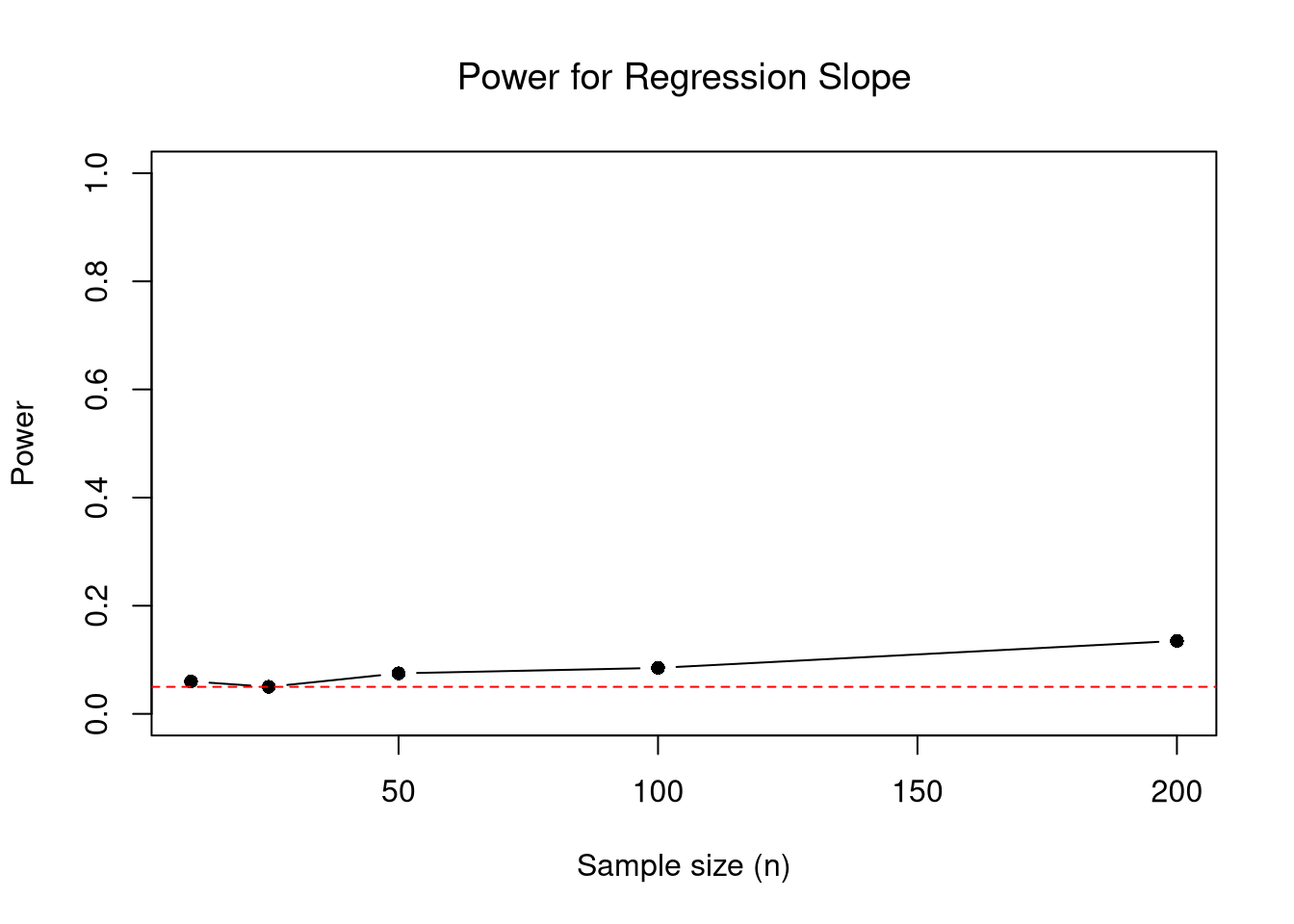
There is an important Trade-off for fixed sample sizes: Increasing significance (fewer false positive) often lowers power (more false negatives). Generally, power depends on the effect size and sample size: bigger true effects and larger \(n\) make it easier to detect real differences (higher power, lower \(\beta\)).
Regression Slope Example.
Continuing the USArrests regression, consider testing \(H_0: \beta_1 = 0\). We can simulate Type I and Type II error rates by generating data that resemble the original. When the true slope is \(0\) (null is true), rejecting is a Type I Error. When the true slope is nonzero (null is false), failing to reject is a Type II Error.
Code
# DGP calibrated to USArrests regressionbeta0 <-coef(reg)[1]beta1_true <-coef(reg)[2]sigma_e <-summary(reg)$sigmax_mean <-mean(xy[, 'x'])x_sd <-sd(xy[, 'x'])# Function: simulate data, return theoretical p-value for slopesim_pval <-function(n, beta1) { X <-rnorm(n, mean = x_mean, sd = x_sd) Y <- beta0 + beta1 * X +rnorm(n, 0, sigma_e)summary(lm(Y ~ X))$coefficients[2, 4]}sim_reps <-200alpha <-0.05# Type I Error rate: true slope = 0pvals_null <-replicate(sim_reps, sim_pval(n =50, beta1 =0))type1_rate <-mean(pvals_null < alpha)type1_rate # should be close to alpha## [1] 0.025# Power: true slope = beta1_truepvals_alt <-replicate(sim_reps, sim_pval(n =50, beta1 = beta1_true))power_est <-mean(pvals_alt < alpha)power_est## [1] 0.055
Code
# Power increases with sample sizen_grid <-c(10, 25, 50, 100, 200)power_by_n <-sapply(n_grid, function(ni) { pvals <-replicate(sim_reps, sim_pval(ni, beta1 = beta1_true))mean(pvals < alpha)})plot(n_grid, power_by_n, type ='b', pch =16,xlab ='Sample size (n)', ylab ='Power',ylim =c(0, 1),main =NA)title('Power for Regression Slope', font.main =1)abline(h = alpha, lty =2, col =rgb(1, 0, 0, .8))
17.3 Bayesian Updating
Bayes’ Theorem.
Bayes’ theorem maps predictive statements into inferential statements. In bivariate form, \[\begin{eqnarray}
Prob(X_i=x \mid Y_i=y)
&=&
\frac{Prob(Y_i=y \mid X_i=x)Prob(X_i=x)}{Prob(Y_i=y)}.
\end{eqnarray}\]
Interpretation:
\(Prob(X_i=x)\) is the prior probability for \(X_i=x\).
\(Prob(Y_i=y|X_i=x)\) is the likelihood of seeing \(Y_i=y\) if \(X_i=x\) is true.
\(Prob(X_i=x|Y_i=y)\) is the posterior, your updated probability after seeing \(Y_i=y\).
A useful way to remember this is \[\begin{eqnarray}
\text{Posterior} \propto \text{Likelihood} \times \text{Prior}.
\end{eqnarray}\] For two states, posterior odds are prior odds times a likelihood ratio.
Building on the coin-flip examples from the previous chapter, suppose we observe the outcome of the second coin (\(Y_i\)) and want to update our belief about the first coin (\(X_i\)).
NoteMust Know
Fair coins. With \(Prob(X_i=x,Y_i=y)=1/4\) for all \(x,y\in\{0,1\}\), the prior is \(Prob(X_i=1)=1/2\) and the likelihoods are \[\begin{eqnarray}
Prob(Y_i=1|X_i=1)=1/2,\quad Prob(Y_i=1|X_i=0)=1/2.
\end{eqnarray}\] Applying Bayes’ theorem, \[\begin{eqnarray}
Prob(X_i=1|Y_i=1)
&=& \frac{Prob(Y_i=1|X_i=1)Prob(X_i=1)}{Prob(Y_i=1)}
= \frac{(1/2)(1/2)}{1/2} = \frac{1}{2}.
\end{eqnarray}\] The posterior equals the prior because the coins are independent — seeing one coin tells you nothing about the other.
Unfair coins. Now consider the joint distribution from the previous chapter with probs <- c(0.4, 0.2, 0.1, 0.3):
\(x=0\)
\(x=1\)
Marginal
\(y=0\)
\(0.4\)
\(0.1\)
\(0.5\)
\(y=1\)
\(0.2\)
\(0.3\)
\(0.5\)
Marginal
\(0.6\)
\(0.4\)
\(1\)
The prior is \(Prob(X_i=1)=0.4\). The likelihoods are \[\begin{eqnarray}
Prob(Y_i=1|X_i=1) = \frac{0.3}{0.4} = 0.75,\quad
Prob(Y_i=1|X_i=0) = \frac{0.2}{0.6} = \frac{1}{3}.
\end{eqnarray}\] Applying Bayes’ theorem, \[\begin{eqnarray}
Prob(X_i=1|Y_i=1)
&=& \frac{0.75 \times 0.4}{0.75 \times 0.4 + \frac{1}{3}\times 0.6}
= \frac{0.3}{0.3+0.2} = 0.6.
\end{eqnarray}\] The prior probability of heads on the first coin was \(0.4\), but after seeing heads on the second coin, it increases to \(0.6\). The coins are not independent: when the second coin shows heads, it is more likely that the first coin also shows heads.
Suppose a screening test has sensitivity 0.90 and false positive rate 0.08, while prevalence is 0.12: \[\begin{eqnarray}
Prob(Y_i=1|X_i=1)=0.90,\quad
Prob(Y_i=1|X_i=0)=0.08,\quad
Prob(X_i=1)=0.12,
\end{eqnarray}\] where \(X_i=1\) means “condition present” and \(Y_i=1\) means “test positive”.
Then \[\begin{eqnarray}
Prob(X_i=1|Y_i=1)
&=&
\frac{0.90\times0.12}{0.90\times0.12 + 0.08\times0.88}
\approx 0.605.
\end{eqnarray}\] Even with a good test, posterior probability depends strongly on prevalence.
Code
# States: X in {0, 1}, signal Y in {0, 1}# Prior Prob(X_i=1)p_x1 <-0.12# Test characteristicsp_y1_x1 <-0.90p_y1_x0 <-0.08# Law of total probability for Prob(Y_i=1)p_y1 <- p_y1_x1 * p_x1 + p_y1_x0 * (1- p_x1)# Bayes posterior Prob(X_i=1 | Y_i=1)p_x1_y1 <- (p_y1_x1 * p_x1) / p_y1p_x1_y1## [1] 0.6053812# Also compute Prob(X_i=1 | Y_i=0)p_y0_x1 <-1- p_y1_x1p_y0_x0 <-1- p_y1_x0p_y0 <- p_y0_x1 * p_x1 + p_y0_x0 * (1- p_x1)p_x1_y0 <- (p_y0_x1 * p_x1) / p_y0p_x1_y0## [1] 0.01460565
Regression Slope Example.
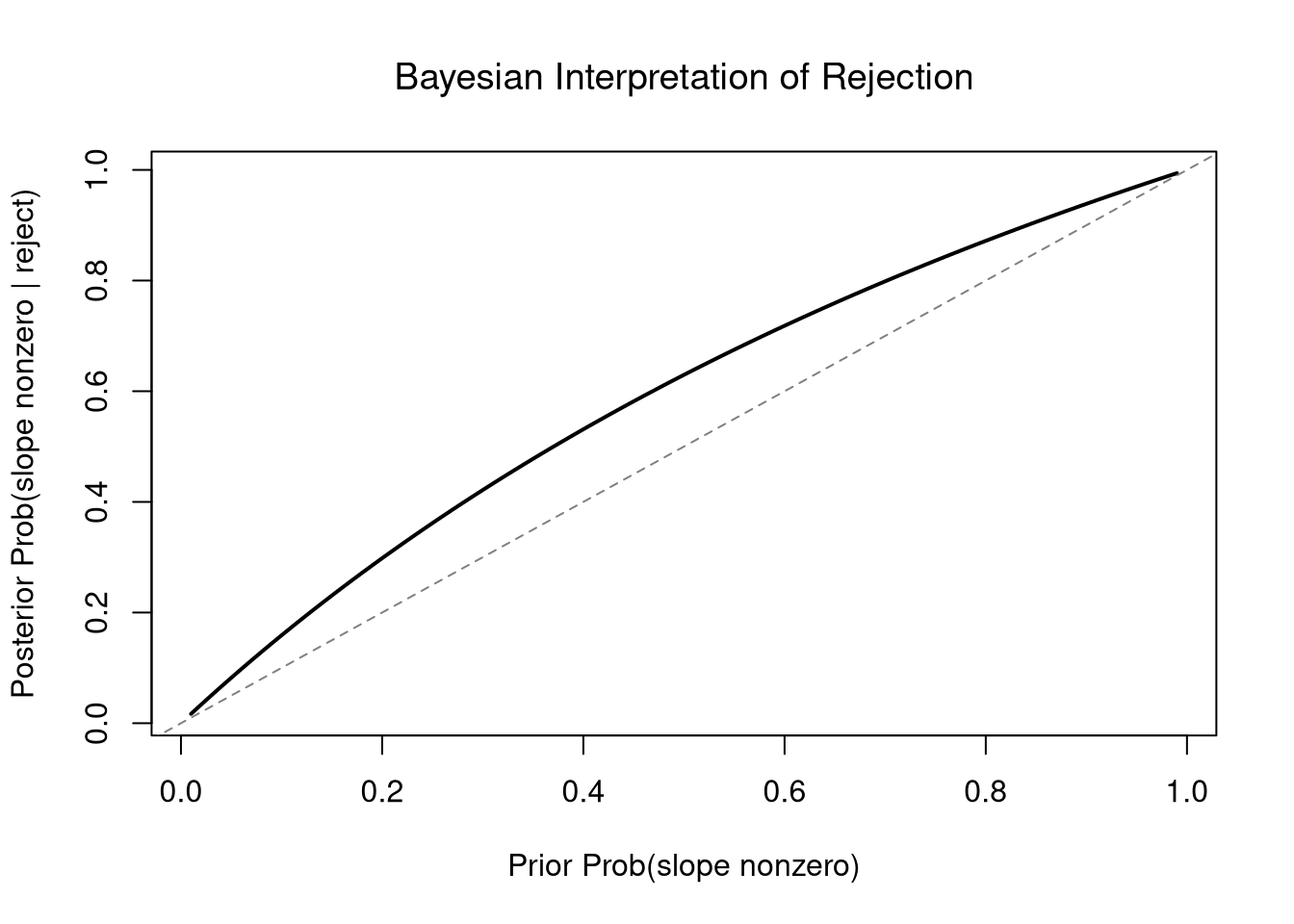
The screening test has the same structure as testing a regression slope. Let \(X_i=1\) mean “slope is truly nonzero” and \(Y_i=1\) mean “the test rejects \(H_0\).” Then sensitivity equals power, the false positive rate equals \(\alpha\), and prevalence is your prior belief that the slope is nonzero. Using the simulation results from the previous section:
Even with moderate power, a rejection substantially updates the posterior probability that the slope is nonzero. A weaker prior (e.g., \(Prob(\beta_1 \neq 0) = 0.1\)) would require stronger evidence to reach the same posterior.
Code
# How the posterior changes with different priorsprior_grid <-seq(0.01, 0.99, by =0.01)post_grid <- (power_est * prior_grid) / (power_est * prior_grid + alpha * (1- prior_grid))plot(prior_grid, post_grid, type ='l', lwd =2,xlab ='Prior Prob(slope nonzero)',ylab ='Posterior Prob(slope nonzero | reject)',main =NA)title('Bayesian Interpretation of Rejection', font.main =1)abline(0, 1, lty =2, col =grey(0.5))
17.4 Exercises
Explain the difference between a Type I Error and a Type II Error in the context of testing \(H_0: \beta_1 = 0\) for a regression slope. Why does increasing the sample size \(n\) improve power without changing the significance level \(\alpha\)?
A screening test has sensitivity \(Prob(Y_i=1|X_i=1) = 0.95\), false positive rate \(Prob(Y_i=1|X_i=0) = 0.10\), and prevalence \(Prob(X_i=1) = 0.05\). Use Bayes’ theorem to compute the posterior probability \(Prob(X_i=1|Y_i=1)\). Explain why the posterior is much lower than the sensitivity.
Using the USArrests dataset, regress Murder on UrbanPop with lm. Extract the theoretical \(t\)-statistic and \(p\)-value for the slope from summary(). Then write a bootstrap loop with \(B = 399\) replicates to compute a bootstrap \(p\)-value and compare it to the theoretical one.
Further Reading.
Many introductory econometrics textbooks have a good appendix on probability and statistics. See also the further reading in Bivariate Probability.
Let each group \(g\) have median \(\tilde{M}_{g}\), interquartile range \(\hat{IQR}_{g}\), observations \(n_{g}\). We can compute standard deviation of the median as \(\tilde{S}_{g}= \frac{1.25 \hat{IQR}_{g}}{1.35 \sqrt{n_{g}}}\). As a rough guess, the interval \(\tilde{M}_{g} \pm 1.7 \tilde{S}_{g}\) is the historical default and displayed as a notch in the boxplot. See also https://www.tandfonline.com/doi/abs/10.1080/00031305.1978.10479236.↩︎