15  Inference & Prediction


15.1 Variability

Often, we are interested in gradients: how \(Y\) changes with \(X\). The linear model depicts this as a simple constant, \(\hat{b}_{1}\), whereas other models do not. A great first step to assess gradients is to plot the predicted values over the explanatory values. A great second step is to compute gradients and summarize them. In any case, we compute confidence intervals to account for variability across samples.

Confidence Bands.

We can construct confidence bands using the jackknife or bootstrap.

Code
## Data
library("wooldridge")
dat <- wage1[order(wage1[,'educ']), c('wage','educ')]

# Loess
reg_lo <- loess(wage~educ, data=dat, span=.8)

# Predictions at design points
pred_design <- data.frame(educ=unique(dat[,'educ']))
preds_lo <- predict(reg_lo, newdata=pred_design)

# Plot
lo_col <- hcl.colors(3,alpha=.5)[2]
plot(wage~educ, pch=16, col=grey(0,.1), data=dat)
lines(pred_design[,'educ'], preds_lo,
    col=lo_col,
    type='o', pch=2)

# Boot CI
boot_lo <- sapply(1:399, function(b){
    # xy_i <- xy[-i,] #jackknife for i in 1:nrow(xy)
    xy_b <- dat[sample(nrow(dat), replace=T),]
    reg_b <- loess(wage~educ, dat=xy_b, span=.8)
    predict(reg_b, newdata=pred_design)
})
boot_cb <- apply(boot_lo,1, quantile,
    probs=c(.025,.975), na.rm=T)


# Plot CI
polygon(
    c(pred_design[[1]], rev(pred_design[[1]])),
    c(boot_cb[1,], rev(boot_cb[2,])),
    col=lo_col,
    border=NA)

Construct a bootstrap confidence band for the following loess regression

Code
# Adaptive-width subsamples with non-uniform weights
xy <- USArrests[,c('UrbanPop','Murder')]
xy0 <- xy[order(xy[,'UrbanPop']),]
names(xy0) <- c('x','y')

plot(y~x, pch=16, col=grey(0,.5), dat=xy0)
reg_lo2 <- loess(y~x, data=xy0, span=.6)

red_col <- rgb(1,0,0,.5)
lines(xy0[,'x'], predict(reg_lo2),
    col=red_col, type='o', pch=2)

Gradients.

There are two ways to summarize gradients

  1. For all methods, including regressograms, you can approximate gradients with small finite differences. For some small difference \(d\), we can manually compute \[\begin{eqnarray} \hat{b}_{1}(x) &=& \frac{ \hat{y}(x+\frac{d}{2}) - \hat{y}(x-\frac{d}{2})}{d}, \end{eqnarray}\]

  2. When using split-sample regressions or local linear regressions, you can use the estimated slope coefficients \(\hat{b}_{1}(x)\) as gradient estimates in each direction.

After computing gradients, you can summarize them in various plots. These plots show variability within-sample, in contrast to the confidence band which shows variability across samples.

Code
## Gradients
pred_lo <- predict(reg_lo)
grad_x  <- dat[,'educ'][-1]
grad_dx <- diff(dat[,'educ'])
grad_dy <- diff(pred_lo)
grad_lo <-grad_dy/grad_dx

## Visual Summary
par(mfrow=c(1,2))
hist(grad_lo,  breaks=20,
    border=NA, freq=F,
    col=lo_col,
    xlab=expression(d~hat(y)/dx),
    main='') ## Distributional Summary
plot(grad_x+grad_dx, grad_lo,
    xlab='x', ylab=expression(d~hat(y)/dx),
    col=lo_col, pch=16) ## Diminishing Returns?

You may also be interested in a particular gradient or a single summary statistic. For example, a bivariate regressogram can estimate the “marginal effect at the mean”; \(\hat{b}_{1}( x=\hat{M}_{X} )\). More typically, you would be interested in the “mean of the gradients”, sometimes said simply as “average effect”, which averages the gradients over all datapoints in the dataset: \(1/n \sum_{i}^{n} \hat{b}_{1}(x=\hat{X}_{i})\). Alternatively, you may be interested in the median of the gradients, or measures of “effect heterogeneity”: the interquartile range or standard deviation of the gradients. Such statistics are single numbers that can be presented in tabular form: “mean gradient (sd gradient)”. You can also report standard errors: “mean gradient (estimated se), sd gradient (estimated se)”.

Code
## Tabular Summary
tab_stats <- c(
    Mean=mean(grad_lo, na.rm=T),
    SD=sd(grad_lo, na.rm=T))

## Use bootstrapping to get SE's
boot_stats <- matrix(NA, nrow=299, ncol=2)
colnames(boot_stats) <- c('Mean SE', 'SD SE')
for(b in 1:nrow(boot_stats)){
    xy_b <- dat[sample(1:nrow(dat), replace=T),]
    reg_lo <- loess(wage~educ, data=xy_b, span=.6)
    pred_lo <- predict(reg_lo)
    grad_lo <- diff(pred_lo)/diff(xy_b[,'educ'])
    dydx_mean <- mean(grad_lo, na.rm=T)
    dydx_sd <- sd(grad_lo, na.rm=T)
    boot_stats[b,1] <- dydx_mean
    boot_stats[b,2] <- dydx_sd
}
boot_se <- apply(boot_stats, 2, sd)

## Printing
tab_regstyle <- data.frame(
  Estimate  = round(tab_stats, 3),
  SE = paste0('(', round(boot_se, 3), ')')
)
tab_regstyle
##      Estimate      SE
## Mean    0.449 (0.071)
## SD      0.531 (0.088)
Summary of Local Gradients
Summary.Statistic Estimate Bootstrap.SE
Mean 0.449 0.071
SD 0.531 0.088

15.2 Theory

Confidence Bands.

Note that confidence bands are approximations to what we want: how much do the predicted values vary from sample to sample.

To make that clear, we will use a simulation where we can actually generate different samples.

Code
## Ages
Xmx <- 70
Xmn <- 15

##Generate Sample Data
dat_sim <- function(n=1000){
    n  <- 1000
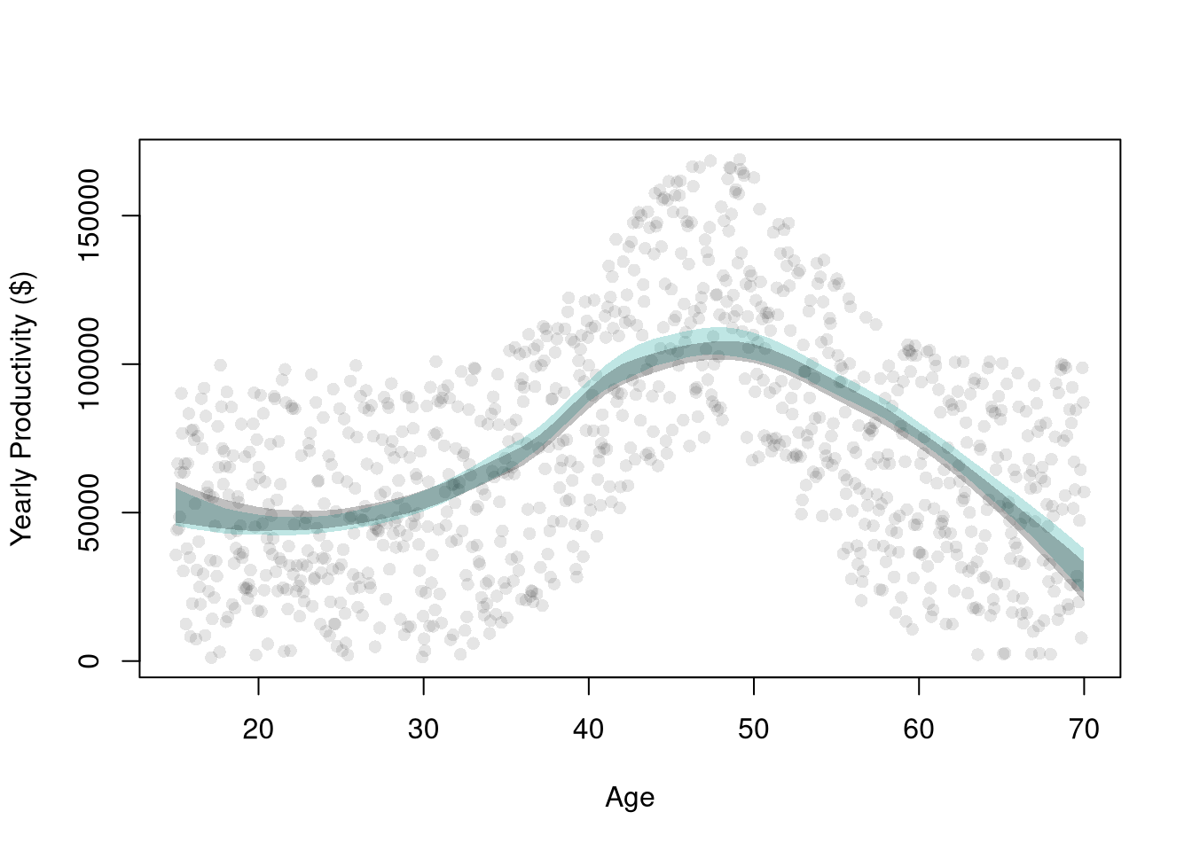
    X <- seq(Xmn,Xmx,length.out=n)
    ## Random Productivity
    e <- runif(n, 0, 1E6)
    beta <-  1E-10*exp(1.4*X -.015*X^2)
    Y    <-  (beta*X + e)/10
    return(data.frame(Y,X))
}
dat0 <- dat_sim(1000)
dat0 <- dat0[order(dat0[,'X']),]

## Data from one sample
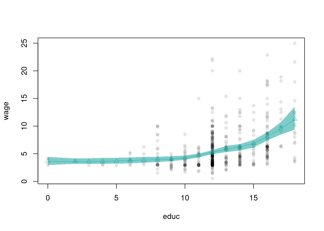
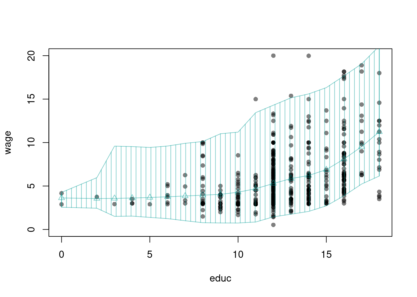
plot(Y~X, data=dat0, pch=16, col=grey(0,.1),
    ylab='Yearly Productivity ($)', xlab='Age' )
reg_lo <- loess(Y~X, data=dat0, span=.8)

## Plot Bootstrap CI for Single Sample
pred_design <- data.frame(X=seq(Xmn, Xmx))
preds_lo <- predict(reg_lo, newdata=pred_design)
boot_lo <- sapply(1:399, function(b){
    dat0_i <- dat0[sample(nrow(dat0), replace=T),]
    reg_i <- loess(Y~X, dat=dat0_i, span=.8)
    predict(reg_i, newdata=pred_design)
})
boot_cb <- apply(boot_lo,1, quantile,
    probs=c(.025,.975), na.rm=T)
polygon(
    c(pred_design[[1]], rev(pred_design[[1]])),
    c(boot_cb[1,], rev(boot_cb[2,])),
    col=hcl.colors(3,alpha=.25)[2],
    border=NA)

# Construct CI across Multiple Samples
sample_lo <- sapply(1:399, function(b){
    xy_b <- dat_sim(1000) #Entirely new sample
    reg_b <- loess(Y~X, dat=xy_b, span=.8)
    predict(reg_b, newdata=pred_design)
})
ci_lo <- apply(sample_lo,1, quantile,
    probs=c(.025,.975), na.rm=T)
polygon(
    c(pred_design[[1]], rev(pred_design[[1]])),
    c(ci_lo[1,], rev(ci_lo[2,])),
    col=grey(0,alpha=.25),
    border=NA)

Variance (Diminishing Returns).

Just as before, there are diminishing returns to larger sample sizes for bivariate statistics. For example, the slope coefficient in simple OLS varies less from sample to sample when the samples are larger. Same for the gradients in loess. This decreased variability across samples makes hypothesis testing more accurate.

Code
B <- 300
Nseq <- seq(10,50, by=1)
SE <- sapply(Nseq, function(n){
    sample_stat <- sapply(1:B, function(b){
        x <- rnorm(n)
        e <- rnorm(n)
        y <- x*3 + x + e
        reg_lo <- loess(y~x)
        pred_lo <- predict(reg_lo)
        grad_lo <- diff(pred_lo)/diff(x)
        dydx_mean <- mean(grad_lo, na.rm=T)
        #dydx_sd <- sd(grad_lo, na.rm=T)
        return(dydx_mean)
    })
    sd(sample_stat)
})

plot(Nseq, SE, pch=16, col=grey(0,.5),
    main='Mean gradient', font.main=1,
    ylab='standard error',
    xlab='sample size')

Bias vs. Variance.

Model choice is a bias-variance tradeoff.

  • High-bias / low-variance models (e.g., strict linear models) are stable across samples but can miss curvature.
  • Low-bias / high-variance models (e.g., very flexible local fits) can capture curvature but may overfit noise.

To formalize the idea, let \(\hat{m}(x)\) be the model prediction for the true conditional mean \(m(x)=E[Y|X=x]\). At each \(x\), prediction error can be decomposed as \[\begin{eqnarray} E\left[(\hat{m}(x)-m(x))^2\right] = \underbrace{\left(E[\hat{m}(x)]-m(x)\right)^2}_{\text{Bias}^2} + \underbrace{Var(\hat{m}(x))}_{\text{Variance}}. \end{eqnarray}\] This equation is useful because it shows why “more flexible” is not always “better”.

Code
set.seed(123)

# True data generating process (nonlinear)
true_m <- function(x) { 1 + 0.8*x - 0.25*x^2 + 0.15*x^3 }
x0 <- seq(-2, 2, length.out=120)
m0 <- true_m(x0)

B <- 300
n <- 80

# Storage for predictions at common x-grid
pred_lm <- matrix(NA_real_, nrow=length(x0), ncol=B)
pred_lo_smooth <- matrix(NA_real_, nrow=length(x0), ncol=B)  # higher bias, lower variance
pred_lo_flex <- matrix(NA_real_, nrow=length(x0), ncol=B)    # lower bias, higher variance

for(b in 1:B){
  x <- sort(runif(n, min=-2, max=2))
  y <- true_m(x) + rnorm(n, sd=0.8)
  sim_dat <- data.frame(x=x, y=y)

  fit_lm <- lm(y~x, data=sim_dat)
  fit_lo_s <- loess(y~x, data=sim_dat, span=0.9)
  fit_lo_f <- loess(y~x, data=sim_dat, span=0.3)

  pred_lm[,b] <- predict(fit_lm, newdata=data.frame(x=x0))
  pred_lo_smooth[,b] <- predict(fit_lo_s, newdata=data.frame(x=x0))
  pred_lo_flex[,b] <- predict(fit_lo_f, newdata=data.frame(x=x0))
}

# Pointwise bias^2 and variance
mean_pred <- function(P) rowMeans(P, na.rm=TRUE)
var_pred <- function(P) apply(P, 1, var, na.rm=TRUE)
avg_bias2 <- function(P) mean((mean_pred(P) - m0)^2, na.rm=TRUE)
avg_var   <- function(P) mean(var_pred(P), na.rm=TRUE)

metrics <- rbind(
  c(avg_bias2(pred_lm),        avg_var(pred_lm)),
  c(avg_bias2(pred_lo_smooth), avg_var(pred_lo_smooth)),
  c(avg_bias2(pred_lo_flex),   avg_var(pred_lo_flex))
)
colnames(metrics) <- c("Avg Bias^2", "Avg Variance")
rownames(metrics) <- c("Linear", "Loess span=0.9", "Loess span=0.3")
round(metrics, 4)
##                Avg Bias^2 Avg Variance
## Linear             0.1267       0.0189
## Loess span=0.9     0.0035       0.0281
## Loess span=0.3     0.0004       0.0837

You can also visualize the three average fits against the true curve:

Code
m_lm <- rowMeans(pred_lm, na.rm=TRUE)
m_lo_s <- rowMeans(pred_lo_smooth, na.rm=TRUE)
m_lo_f <- rowMeans(pred_lo_flex, na.rm=TRUE)

y_rng <- range(c(m0, m_lm, m_lo_s, m_lo_f), na.rm=TRUE)
plot(x0, m0, type='l', lwd=2, col=1, ylim=y_rng,
  xlab="x", ylab="E[Y|X]", main="")
lines(x0[is.finite(m_lm)], m_lm[is.finite(m_lm)], lwd=2, col=2)
lines(x0[is.finite(m_lo_s)], m_lo_s[is.finite(m_lo_s)], lwd=2, col=4)
lines(x0[is.finite(m_lo_f)], m_lo_f[is.finite(m_lo_f)], lwd=2, col=3)
legend("topleft", lty=1, lwd=2, col=c(1,2,4,3),
  legend=c("True mean", "Linear", "Loess span=0.9", "Loess span=0.3"))

In practice, compare models with cross-validation (below). The preferred model is the one with best out-of-sample performance, not the one with the most flexible in-sample fit.

15.3 Prediction

Describe vs. Explain vs. Predict.

Understanding whether we aim to describe, explain, or predict is central to empirical analysis. The three distinct purposes are to accurately describe empirical patterns, explain why the empirical patterns exist, predict what empirical patterns will exist.

Objective Core Question Goal Methods
Describe What is happening? Characterize patterns & facts Summary stats, visualizations, correlations
Explain Why is it happening? Establish causal relationships & mechanisms Theoretical models; experimentation; counterfactual reasoning
Predict What will happen? Anticipate outcomes; support decisions that affect the future Machine learning, treatment effect forecasting, policy simulations

Here is an example for minimum wages.

  • Describe: Studies document that following minimum-wage increases, overall low-wage employment may look roughly stable in the short run, but disaggregated data often show larger employment declines over longer horizons, especially among youths and racial minorities.
  • Explain: Studies investigate economic mechanisms such as (i) whether lower productivity populations are more vulnerable and employers adjust along hiring margins (fewer openings, higher required skills), and (ii) whether effects are larger in sectors like retail/food service where minimum wages bite hardest.
  • Predict: A policy simulation that raises the wage floor incorporates subgroup-specific elasticities to forecast different employment losses (e.g., unemployment for teenage or black workers and income gains for stayers)

The distinctions matter, as they help you recognize that predictive accuracy or good data visualization does not equal causal insight. You can then better align statistical tools with questions. Try remembering this: Describe reality, Explain causes, Predict futures

Prediction Intervals.

Here, we consider a range for \(Y_{i}\) rather than for \(m(X_{i})\). These intervals also take into account the residuals, the variability of individuals rather than the variability of their mean.

Code
# Bivariate Data from USArrests
xy <- USArrests[,c('Murder','UrbanPop')]
colnames(xy) <- c('y','x')
xy0 <- xy[order(xy[,'x']),]

For a nice overview of different types of intervals, see https://www.jstor.org/stable/2685212. For an in-depth view, see “Statistical Intervals: A Guide for Practitioners and Researchers” or “Statistical Tolerance Regions: Theory, Applications, and Computation”. See https://robjhyndman.com/hyndsight/intervals/ for constructing intervals for future observations in a time-series context. See Davison and Hinkley, chapters 5 and 6 (also Efron and Tibshirani, or Wehrens et al.)

Code
# Design Points
X0 <- unique(dat[,'educ'])
# Regression
reg_lo <- loess(wage~educ, data=dat, span=.8)
preds_lo <- predict(reg_lo, newdata=data.frame(educ=X0))

# Bootstrap Residuals
n <- nrow(dat)
res_lo <- lapply(1:399, function(i){
    dat_b <- dat[sample(n, replace=T),]
    reg_b <- loess(wage~educ, dat=dat_b, span=.8)
    resids_b <- resid(reg_b)
    cbind(e=resids_b, educ=dat_b[,'educ'])
})
res_lo <- do.call(rbind, res_lo)

## Smooth residuals
res_fun <- function(x0, h){
    # Include only residuals within h distance to x0
    ki0 <- abs(res_lo[,'educ']-x0)/h
    ki0 <- dunif(ki0)/h
    ei0 <- res_lo[ki0 != 0, 'e'] #subset estimates   
    ## Local quantiles
    res_i <- quantile(ei0, probs=c(.025,.975), na.rm=T)
    res_i
}
res_ci <- sapply(X0, res_fun, h=5)

## Prediction Interval
pi_lo1 <- preds_lo + res_ci[1,]
pi_lo2 <- preds_lo + res_ci[2,]

#Plot
col <- hcl.colors(3,alpha=.5)[2]
plot(wage~educ, pch=16, col=grey(0,.5),
    dat=dat, ylim=c(0, 20))
lines(X0, preds_lo,
    col=col, type='o', pch=2)
polygon( c(X0, rev(X0)),
    c(pi_lo1, rev(pi_lo2)),
    col=col, density=12, angle=90)

Consider also this example below with a linear model. Expand on it by using the Normal Approximation for the residuals (hint: use qnorm).

Code
reg <- lm(wage~educ, dat=dat)

# Bootstrap Prediction Interval
boot_resids <- lapply(1:399, function(b){
    b_id <- sample( nrow(dat), replace=T)
    dat_b <- dat[b_id,]
    reg_b <- lm(wage~educ, dat=dat_b)
    e_b <- resid(reg_b)
    x_b <- reg_b[['model']][['educ']]
    res_b <- cbind(e_b, x_b)
})
boot_resids <- as.data.frame(do.call(rbind, boot_resids))

# Errors do not vary with x
ehat <- quantile(boot_resids[,'e_b'], probs=c(.025, .975))

# PI
phat <- predict(reg)
boot_pi <- cbind(phat + ehat[1], phat + ehat[2])

# Plot Bootstrap PI
plot(wage~educ, dat=dat, pch=16, main='Prediction Intervals',
    ylim=c(-5,20), font.main=1)
x <- dat[,'educ']
lines(x, phat, type='o', pch=2)
polygon( c(x, rev(x)),
    c(boot_pi[,1], rev(boot_pi[,2])),
    col=grey(0,.2), border=NA)

Code

# Normal PI (Make by hand)
#pi <- predict(reg, interval='prediction')
#lines( x, pi[,'lwr'], lty=2)
#lines( x, pi[,'upr'], lty=2)

Cross Validation.

Perhaps the most common approach to selecting a bandwidth is to minimize error. Leave-one-out Cross-validation minimizes the average “leave-one-out” mean square prediction errors: \[\begin{eqnarray} \min_{h} \quad \frac{1}{n} \sum_{i=1}^{n} \left[ \hat{Y}_{i} - \hat{y_{[i]}}(X,h) \right]^2, \end{eqnarray}\] where \(\hat{y}_{[i]}(X,h)\) is the model predicted value at \(X_{i}\) based on a dataset that excludes \(X_{i}\), and \(h\) is the bandwidth (e.g., bin size in a regressogram).

Minimizing out-sample prediction error is perhaps the simplest computational approach to choose bandwidths, and it also addresses an issue that plagues observational studies in the social sciences: your model explains everything and predicts nothing. Note, however, minimizing prediction error is not objectively “best”.

Code
library(wooldridge)
# Crossvalidated bandwidth for regression
xy_mat <- data.frame(x=wage1[,'educ'], y=wage1[,'wage'])

## Grid Search
BWS <- c(0.5,0.6,0.7,0.8)
BWS_CV <- sapply(BWS, function(h){
    E_bw <- sapply(1:nrow(xy_mat), function(i){
        llls <- loess(y~x, data=xy_mat[-i,], span=h,
            degree=1, surface='direct')
        pred_i <- predict(llls, newdata=xy_mat[i,])
        e_i <-  (pred_i- xy_mat[i,'y'])
        return(e_i)
    })
    return( mean(E_bw^2) )
})

## Plot MSE
par(mfrow=c(1,2))
plot(BWS, BWS_CV, ylab='CV error', pch=3,
    xlab='bandwidth (h)')

## Plot Optimal Predictions
h_star <- BWS[which.min(BWS_CV)]
llls <- loess(y~x, data=xy_mat, span=h_star,
    degree=1, surface='direct')
plot(xy_mat, pch=16, col=grey(0,.5),
    xlab='X', ylab='Predictions')

pred_id <- order(xy_mat[,'x'])
lines(xy_mat[pred_id,'x'], predict(llls)[pred_id],
    col=2, lwd=2)