Code
# Bivariate Data from USArrests
xy <- USArrests[,c('Murder','UrbanPop')]
colnames(xy) <- c('y','x')
xy0 <- xy[order(xy[,'x']),]Understanding whether we aim to describe, explain, or predict is central to empirical analysis. The three distinct purposes are to accurately describe empirical patterns, explain why the empirical patterns exist, predict what empirical patterns will exist.
| Objective | Core Question | Goal | Methods |
|---|---|---|---|
| Describe | What is happening? | Characterize patterns & facts | Summary stats, visualizations, correlations |
| Explain | Why is it happening? | Establish causal relationships & mechanisms | Theoretical models; experimentation; counterfactual reasoning |
| Predict | What will happen? | Anticipate outcomes; support decisions that affect the future | Machine learning, treatment effect forecasting, policy simulations |
Here is an example for minimum wages.
The distinctions matter, as they help you recognize that predictive accuracy or good data visualization does not equal causal insight. You can then better align statistical tools with questions. Try remembering this: Describe reality, Explain causes, Predict futures
Here, we consider a range for \(Y_{i}\) rather than for \(m(X_{i})\). These intervals also take into account the residuals, the variability of individuals rather than the variability of their mean.
# Bivariate Data from USArrests
xy <- USArrests[,c('Murder','UrbanPop')]
colnames(xy) <- c('y','x')
xy0 <- xy[order(xy[,'x']),]For a nice overview of different types of intervals, see https://www.jstor.org/stable/2685212. For an in-depth view, see “Statistical Intervals: A Guide for Practitioners and Researchers” or “Statistical Tolerance Regions: Theory, Applications, and Computation”. See https://robjhyndman.com/hyndsight/intervals/ for constructing intervals for future observations in a time-series context. See Davison and Hinkley, chapters 5 and 6 (also Efron and Tibshirani, or Wehrens et al.)
## Data
library("wooldridge")
dat <- wage1[, c('wage','educ')]
dat <- dat[order(wage1[,'educ']), ]


# Design Points
X0 <- unique(dat[,'educ'])
# Regression
reg_lo <- loess(wage~educ, data=dat, span=.8)
preds_lo <- predict(reg_lo, newdata=data.frame(educ=X0))

# Bootstrap Residuals
n <- nrow(dat)
res_lo <- lapply(1:399, function(i){
    dat_b <- dat[sample(n, replace=T),]
    reg_b <- loess(wage~educ, dat=dat_b, span=.8)
    resids_b <- resid(reg_b)
    cbind(e=resids_b, educ=dat_b[,'educ'])
})
res_lo <- do.call(rbind, res_lo)

## Smooth residuals
res_fun <- function(x0, h){
    # Include only residuals within h distance to x0
    ki0 <- abs(res_lo[,'educ']-x0)/h
    ki0 <- dunif(ki0)/h
    ei0 <- res_lo[ki0 != 0, 'e'] #subset estimates
    ## Local quantiles
    res_i <- quantile(ei0, probs=c(.025,.975), na.rm=T)
    res_i
}
res_ci <- sapply(X0, res_fun, h=5)

## Prediction Interval
pi_lo1 <- preds_lo + res_ci[1,]
pi_lo2 <- preds_lo + res_ci[2,]

#Plot
col <- hcl.colors(3,alpha=.5)[2]
plot(wage~educ, pch=16, col=grey(0,.5),
    dat=dat, ylim=c(0, 20))
lines(X0, preds_lo,
    col=col, type='o', pch=2)
polygon( c(X0, rev(X0)),
    c(pi_lo1, rev(pi_lo2)),
    col=col, density=12, angle=90)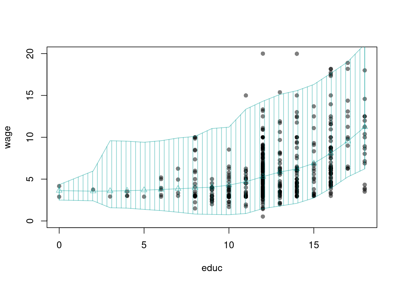
Consider also this example below with a linear model. Expand on it by using the Normal Approximation for the residuals (hint: use qnorm).
reg <- lm(wage~educ, dat=dat)

# Bootstrap Prediction Interval
boot_resids <- lapply(1:399, function(b){
    b_id <- sample( nrow(dat), replace=T)
    dat_b <- dat[b_id,]
    reg_b <- lm(wage~educ, dat=dat_b)
    e_b <- resid(reg_b)
    x_b <- reg_b[['model']][['educ']]
    res_b <- cbind(e_b, x_b)
})
boot_resids <- as.data.frame(do.call(rbind, boot_resids))

# Errors do not vary with x
ehat <- quantile(boot_resids[,'e_b'], probs=c(.025, .975))

# PI
phat <- predict(reg)
boot_pi <- cbind(phat + ehat[1], phat + ehat[2])

# Plot Bootstrap PI
plot(wage~educ, dat=dat, pch=16, main='Prediction Intervals',
    ylim=c(-5,20), font.main=1)
x <- dat[,'educ']
lines(x, phat, type='o', pch=2)
polygon( c(x, rev(x)),
    c(boot_pi[,1], rev(boot_pi[,2])),
    col=grey(0,.2), border=NA)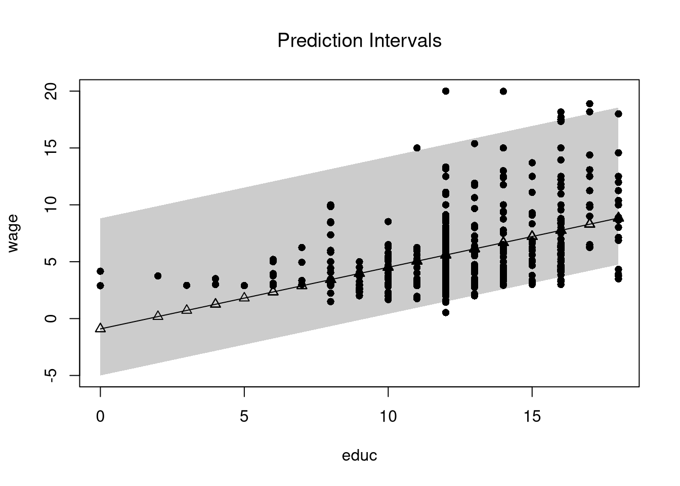
# Normal PI (Make by hand)
#pi <- predict(reg, interval='prediction')
#lines( x, pi[,'lwr'], lty=2)
#lines( x, pi[,'upr'], lty=2)Perhaps the most common approach to selecting a bandwidth is to minimize error. Leave-one-out Cross-validation minimizes the average “leave-one-out” mean square prediction errors: \[\begin{eqnarray} \min_{h} \quad \frac{1}{n} \sum_{i=1}^{n} \left[ \hat{Y}_{i} - \hat{y_{[i]}}(X,h) \right]^2, \end{eqnarray}\] where \(\hat{y}_{[i]}(X,h)\) is the model predicted value at \(X_{i}\) based on a dataset that excludes \(X_{i}\), and \(h\) is the bandwidth (e.g., bin size in a regressogram).
Minimizing out-sample prediction error is perhaps the simplest computational approach to choose bandwidths, and it also addresses an issue that plagues observational studies in the social sciences: your model explains everything and predicts nothing. Note, however, minimizing prediction error is not objectively “best”.
In practice, compare models with cross-validation (below). The preferred model is the one with best out-of-sample performance, not the one with the most flexible in-sample fit.
library(wooldridge)
# Crossvalidated bandwidth for regression
xy_mat <- data.frame(x=wage1[,'educ'], y=wage1[,'wage'])

## Grid Search
BWS <- c(0.5,0.6,0.7,0.8)
BWS_CV <- sapply(BWS, function(h){
    E_bw <- sapply(1:nrow(xy_mat), function(i){
        llls <- loess(y~x, data=xy_mat[-i,], span=h,
            degree=1, surface='direct')
        pred_i <- predict(llls, newdata=xy_mat[i,])
        e_i <-  (pred_i- xy_mat[i,'y'])
        return(e_i)
    })
    return( mean(E_bw^2) )
})

## Plot MSE
par(mfrow=c(1,2))
plot(BWS, BWS_CV, ylab='CV error', pch=3,
    xlab='bandwidth (h)')

## Plot Optimal Predictions
h_star <- BWS[which.min(BWS_CV)]
llls <- loess(y~x, data=xy_mat, span=h_star,
    degree=1, surface='direct')
plot(xy_mat, pch=16, col=grey(0,.5),
    xlab='X', ylab='Predictions')

pred_id <- order(xy_mat[,'x'])
lines(xy_mat[pred_id,'x'], predict(llls)[pred_id],
    col=2, lwd=2)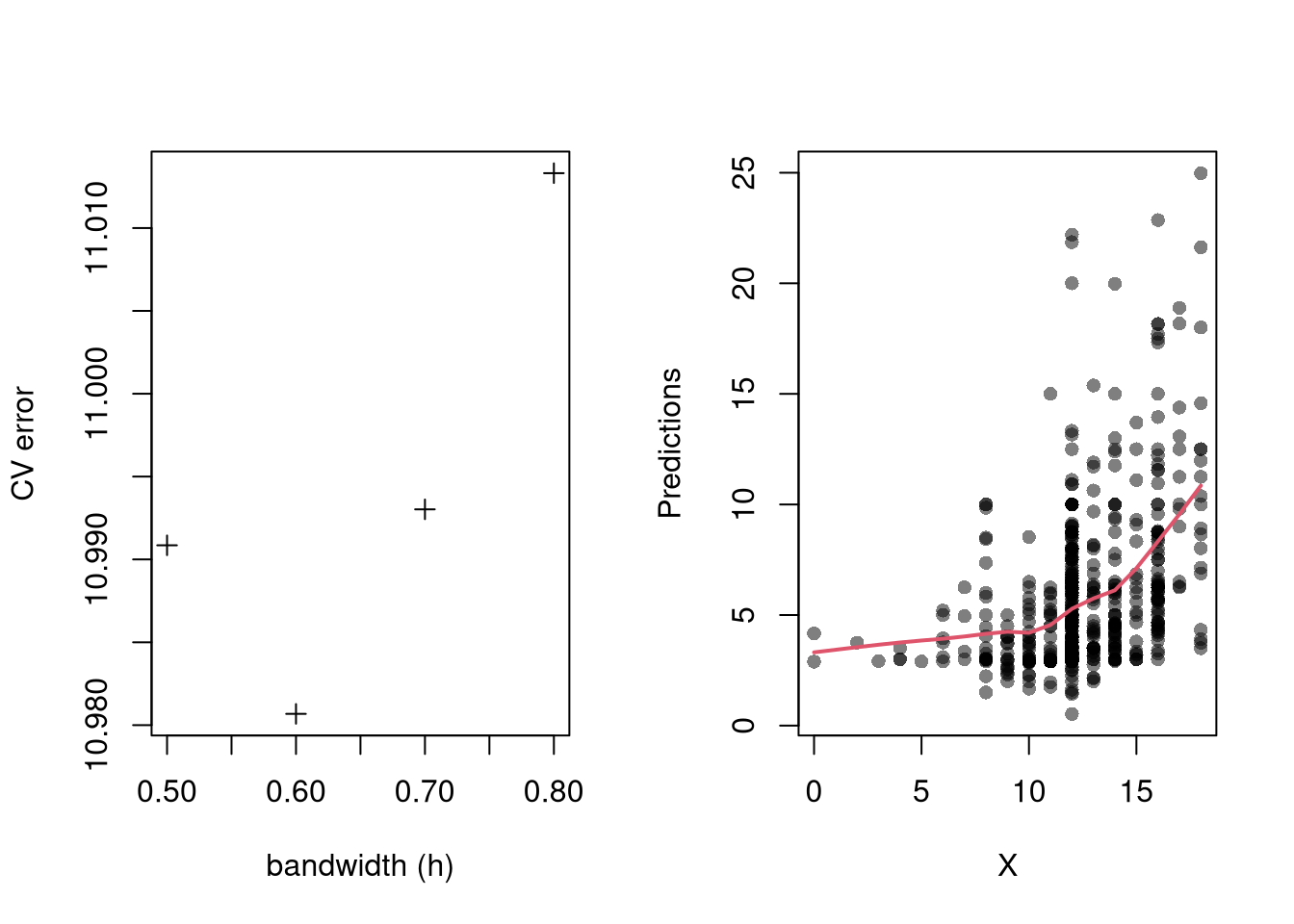
In some cases, we may want to smooth time series data instead of predict into the future. We can distinguish two types of smoothing, incorporating future observations or not. When only weighting two other observations, the differences can be expressed as trying to estimate the average with different available data:
One example of filtering is Exponential Filtering (sometimes confusingly referred to as “Exponential Smoothing”) which weights only previous observations using an exponential kernel.
# Time series data
set.seed(1)
## Underlying Trend
x0 <- cumsum(rnorm(500,0,1))
## Observed Datapoints
x <- x0 + runif(length(x0),-10,10)
dat <- data.frame(t=seq(x), x0=x0, x=x)

## Asymmetric Kernel
#bw <- c(2/3,1/3)
#s1 <- filter(x, bw/sum(bw), sides=1)

## Symmetric Kernel
#bw <- c(1/6,2/3,1/6)
#s2 <- filter(x,  bw/sum(bw), sides=2)
There are several cross-validation procedures for filtering time series data (OpsomerEtAl2001?). One is called time series cross-validation (TSCV), which is useful for temporally dependent data (Hart1991?; HaerdlePhilippe1992?; Bergmeir2018?).
## Plot Simulated Data
x <- dat$x
x0 <- dat$x0
par(fig = c(0,1,0,1), new=F)
plot(x, pch=16, col=grey(0,.25))
lines(x0, col=1, lty=1, lwd=2)

## Work with differenced data?
#n       <- length(Yt)
#plot(Yt[1:(n-1)], Yt[2:n],
#    xlab='d Y (t-1)', ylab='d Y (t)',
#    col=grey(0,.5), pch=16)
#Yt <- diff(Yt)

## TSCV One Sided Moving Average
filter_bws <- seq(1,20,by=1)
filter_mape_bws <- sapply(filter_bws, function(h){
    bw <- c(0,rep(1/h,h)) ## Leave current one out
    s2 <- filter(x, bw, sides=1)
    pe <- s2 - x
    mape <- mean( abs(pe)^2, na.rm=T)
})
filter_mape_star <- filter_mape_bws[which.min(filter_mape_bws)]
filter_h_star <- filter_bws[which.min(filter_mape_bws)]
filter_tscv <- filter(x,  c(rep(1/filter_h_star,filter_h_star)), sides=1)
# Plot Optimization Results
#par(fig = c(0.07, 0.35, 0.07, 0.35), new=T)
#plot(filter_bws, filter_mape_bws, type='o', ylab='mape', pch=16)
#points(filter_h_star, filter_mape_star, pch=19, col=2, cex=1.5)

## TSCV for LLLS
library(np)
llls_bws <- seq(8,28,by=1)
llls_burnin <- 10
llls_mape_bws <- sapply(llls_bws, function(h){ # cat(h,'\n')
    pe <- sapply(llls_burnin:nrow(dat), function(t_end){
        dat_t <- dat[dat$t<t_end, ]
        reg <- npreg(x~t, data=dat_t, bws=h,
            ckertype='epanechnikov',
            bandwidth.compute=F, regtype='ll')
        edat <- dat[dat$t==t_end,]
        pred <- predict(reg, newdata=edat)
        pe <- edat$x - pred
        return(pe)
    })
    mape <- mean( abs(pe)^2, na.rm=T)
})
llls_mape_star <- llls_mape_bws[which.min(llls_mape_bws)]
llls_h_star <- llls_bws[which.min(llls_mape_bws)]
#llls_tscv <- predict( npreg(x~t, data=dat, bws=llls_h_star,
#    bandwidth.compute=F, regtype='ll', ckertype='epanechnikov'))
llls_tscv <- sapply(llls_burnin:nrow(dat), function(t_end, h=llls_h_star){
    dat_t <- dat[dat$t<t_end, ]
    reg <- npreg(x~t, data=dat_t, bws=h,
        ckertype='epanechnikov',
        bandwidth.compute=F, regtype='ll')
    edat <- dat[dat$t==t_end,]
    pred <- predict(reg, newdata=edat)
    return(pred)
})

## Compare Fits Qualitatively
lines(filter_tscv, col=2, lty=1, lwd=1)
lines(llls_burnin:nrow(dat), llls_tscv, col=4, lty=1, lwd=1)
legend('topleft', lty=1, col=c(1,2,4), bty='n',
    c('Underlying Trend', 'MA-1sided + TSCV', 'LLLS-1sided + TSCV'))

## Compare Fits Quantitatively
cbind(
    bandwidth=c(LLLS=llls_h_star, MA=filter_h_star),
    mape=round(c(LLLS=llls_mape_star, MA=filter_mape_star),2) )

## See also https://cran.r-project.org/web/packages/smoots/smoots.pdf
#https://otexts.com/fpp3/tscv.html
#https://robjhyndman.com/hyndsight/tscvexample/Bayes’ theorem maps predictive statements into inferential statements. In bivariate form, \[\begin{eqnarray} Prob(X_i=x \mid Y_i=y) &=& \frac{Prob(Y_i=y \mid X_i=x)Prob(X_i=x)}{Prob(Y_i=y)}. \end{eqnarray}\]
Interpretation:
A useful way to remember this is \[\begin{eqnarray} \text{Posterior} \propto \text{Likelihood} \times \text{Prior}. \end{eqnarray}\] For two states, posterior odds are prior odds times a likelihood ratio.
For a concrete example, suppose a screening test has sensitivity 0.90 and false positive rate 0.08, while prevalence is 0.12: \[\begin{eqnarray} Prob(Y_i=1|X_i=1)=0.90,\quad Prob(Y_i=1|X_i=0)=0.08,\quad Prob(X_i=1)=0.12, \end{eqnarray}\] where \(X_i=1\) means “condition present” and \(Y_i=1\) means “test positive”.
Then \[\begin{eqnarray} Prob(X_i=1|Y_i=1) &=& \frac{0.90\times0.12}{0.90\times0.12 + 0.08\times0.88} \approx 0.605. \end{eqnarray}\] Even with a good test, posterior probability depends strongly on prevalence.
# States: X in {0,1}, signal Y in {0,1}
# Prior Prob(X_i=1)
p_x1 <- 0.12

# Test characteristics
p_y1_x1 <- 0.90
p_y1_x0 <- 0.08

# Law of total probability for Prob(Y_i=1)
p_y1 <- p_y1_x1 * p_x1 + p_y1_x0 * (1 - p_x1)

# Bayes posterior Prob(X_i=1 | Y_i=1)
p_x1_y1 <- (p_y1_x1 * p_x1) / p_y1
p_x1_y1
## [1] 0.6053812

# Also compute Prob(X_i=1 | Y_i=0)
p_y0_x1 <- 1 - p_y1_x1
p_y0_x0 <- 1 - p_y1_x0
p_y0 <- p_y0_x1 * p_x1 + p_y0_x0 * (1 - p_x1)
p_x1_y0 <- (p_y0_x1 * p_x1) / p_y0
p_x1_y0
## [1] 0.01460565Random subsampling is one of many hybrid approaches that tries to combine the best of the core methods: Bootstrap and Jacknife.
| Sample Size per Iteration | Number of Iterations | Resample | |
|---|---|---|---|
| Bootstrap | \(n\) | \(B\) | With Replacement |
| Jackknife | \(n-1\) | \(n\) | Without Replacement |
| Random Subsample | \(m < n\) | \(B\) | Without Replacement |
xy <- USArrests[,c('Murder','UrbanPop')]
colnames(xy) <- c('y','x')
reg <-  lm(y~x, dat=xy)
coef(reg)
## (Intercept)           x
##  6.41594246  0.02093466

# Random Subsamples
rs_regs <- lapply(1:399, function(b){
    b_id <- sample( nrow(xy), nrow(xy)-10, replace=F)
    xy_b <- xy[b_id,]
    reg_b <- lm(y~x, dat=xy_b)
})
rs_coefs <- sapply(rs_regs, coef)['x',]
rs_se <- sd(rs_coefs)

hist(rs_coefs, breaks=25,
    main=paste0('SE est. = ', round(rs_se,4)),
    font.main=1, border=NA,
    xlab=expression(hat(b)[b]))
abline(v=coef(reg)['x'], lwd=2)
rs_ci_percentile <- quantile(rs_coefs, probs=c(.025,.975))
abline(v=rs_ci_percentile, lty=2)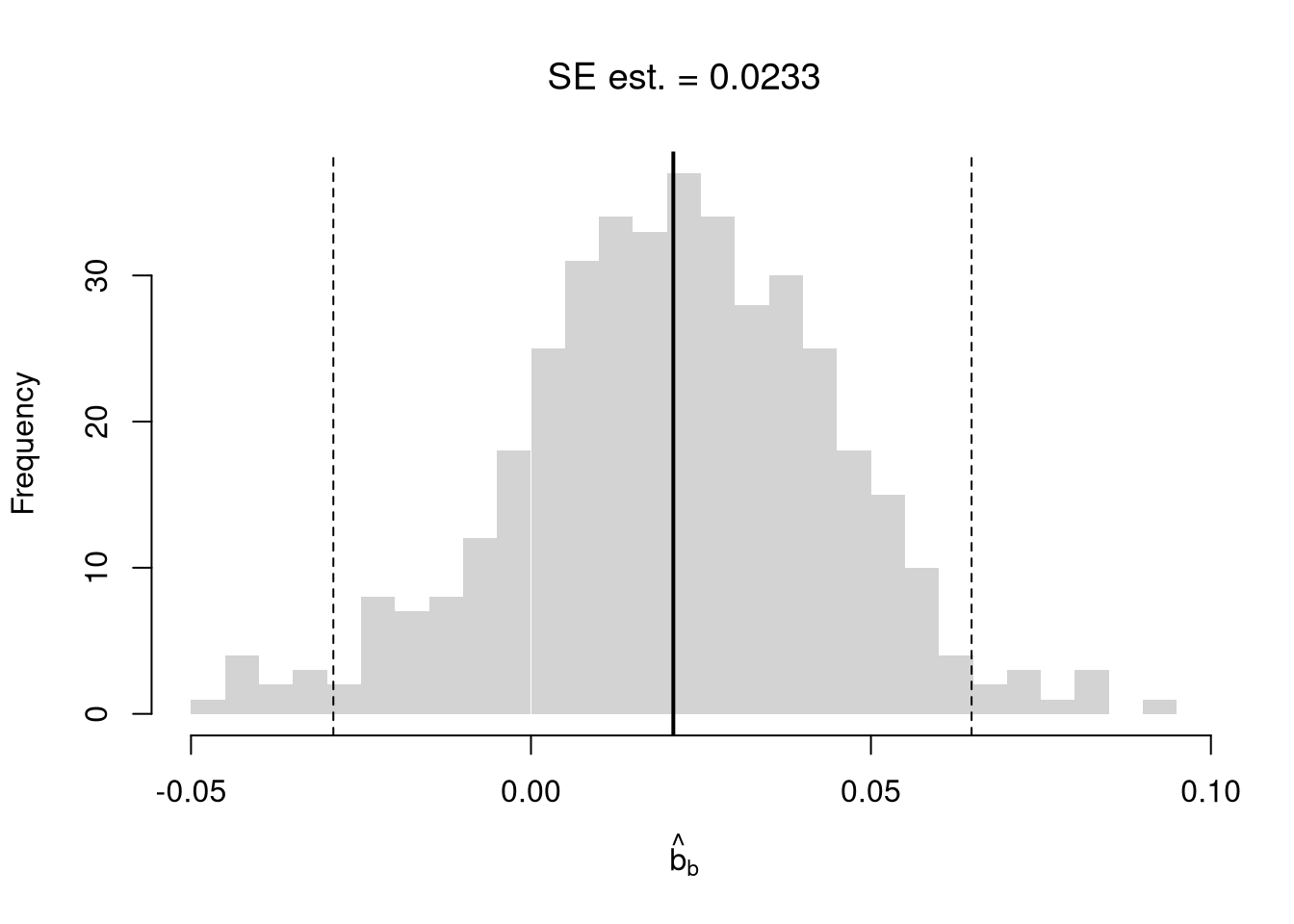
First, not that you can use matrix algebra in R
x_mat1 <- matrix( seq(2,7), 2, 3)
x_mat1
##      [,1] [,2] [,3]
## [1,]    2    4    6
## [2,]    3    5    7

x_mat2 <- matrix( seq(4,-1), 2, 3)
x_mat2
##      [,1] [,2] [,3]
## [1,]    4    2    0
## [2,]    3    1   -1

x_mat1*x_mat2 #NOT classical matrix multiplication
##      [,1] [,2] [,3]
## [1,]    8    8    0
## [2,]    9    5   -7
x_mat1^x_mat2
##      [,1] [,2]      [,3]
## [1,]   16   16 1.0000000
## [2,]   27    5 0.1428571

tcrossprod(x_mat1, x_mat2) #x_mat1 %*% t(x_mat2)
##      [,1] [,2]
## [1,]   16    4
## [2,]   22    7

crossprod(x_mat1, x_mat2)
##      [,1] [,2] [,3]
## [1,]   17    7   -3
## [2,]   31   13   -5
## [3,]   45   19   -7
Second, note that you can apply functions to matrices
sum_squared <- function(x1, x2) {
    y <- (x1 + x2)^2
    return(y)
}
sum_squared(x_mat1, x_mat2)
##      [,1] [,2] [,3]
## [1,]   36   36   36
## [2,]   36   36   36


solve(x_mat1[1:2,1:2])
##      [,1] [,2]
## [1,] -2.5    2
## [2,]  1.5   -1
Third, note that we can conduct OLS regressions efficiently using matrix algebra. Grouping the coefficients as a vector \(B=(b_0 ~~ b_1 ~~... ~~ b_{K})\), we want to find coefficients that minimize the sum of squared errors. The linear model has a fairly simple solution for \(\hat{B}^{*}\) if you know linear algebra. Denoting \(\hat{\mathbf{X}}_{i} = [1~~ \hat{X}_{i1} ~~...~~ \hat{X}_{iK}]\) as a row vector, we can write the model as \(\hat{Y}_{i} = \hat{\mathbf{X}}_{i}B + e_{i}\). We can then write the model in matrix form \[\begin{eqnarray} \hat{Y} &=& \hat{\textbf{X}}B + E \\ \hat{Y} &=& \begin{pmatrix} \hat{Y}_{1} \\ \vdots \\ \hat{Y}_{N} \end{pmatrix} \quad \hat{\textbf{X}} = \begin{pmatrix} 1 & \hat{X}_{11} & ... & \hat{X}_{1K} \\ & \vdots & & \\ 1 & \hat{X}_{n1} & ... & \hat{X}_{nK} \end{pmatrix} \end{eqnarray}\] Minimizing the squared errors: \(\min_{B} e_{i}^2 = \min_{B} (E' E)\), yields coefficient estimates and predictions \[\begin{eqnarray} \hat{B^{*}} &=& (\hat{\textbf{X}}'\hat{\textbf{X}})^{-1}\hat{\textbf{X}}'\hat{Y}\\ \hat{y} &=& \hat{\textbf{X}} \hat{B^{*}} \\ \hat{E} &=& \hat{Y} - \hat{y} \\ \end{eqnarray}\]
# Manually Compute
Y <- USArrests[,'Murder']
X <- USArrests[,c('Assault','UrbanPop')]
X <- as.matrix(cbind(1,X))

XtXi <- solve(t(X)%*%X)
Bhat <- XtXi %*% (t(X)%*%Y)
c(Bhat)
## [1] 3.20715340 0.04390995 -0.04451047With matrix notation, we can established that OLS is an unbiased estimator for additively separable and linear relationships. Assume \[\begin{eqnarray} Y_{i} = X_{i} \beta + \epsilon_{i} &\quad& \mathbb{E}[\epsilon_{i} | X_{i} ]=0, \end{eqnarray}\] then notice that \[\begin{eqnarray} B^{*} = (\mathbf{X}'\mathbf{X})^{-1}\mathbf{X}'Y = (\mathbf{X}'\mathbf{X})^{-1}\mathbf{X}'(\mathbf{X}\beta + \epsilon) = \beta + (X'X)^{-1}X'\epsilon\\ \mathbb{E}\left[ B^{*} \right] = \mathbb{E}\left[ (\mathbf{X}'\mathbf{X})^{-1}\mathbf{X}'Y \right] = \beta + (\mathbf{X}'\mathbf{X})^{-1}\mathbb{E}\left[ \mathbf{X}'\epsilon \right] = \beta \end{eqnarray}\]
If we do not know that the data generating process is additively separable and linear, then we do not know how to interpret \(\hat{B}^{*}\) (outside of a very mathematical expression, which I do not cover here). If we run a local linear regression analysis, on the other hand, we get the estimator \[\begin{eqnarray} \beta(\mathbf{x}) &=& [\mathbf{X}'\mathbf{K}(\mathbf{x})\mathbf{X}]^{-1} \mathbf{X}'\mathbf{K}(\mathbf{x})Y \\ \mathbf{K}(\mathbf{x}) &=& \begin{pmatrix} K\left(\frac{\mathbf{X}_{1}-\mathbf{x}}{h_{1}}\right) & ... & 0\\ \vdots & & \\ 0 & ... & K\left(\frac{\mathbf{X}_{P}-\mathbf{x}}{h_{P}}\right) \end{pmatrix}, \end{eqnarray}\] which is unbiased far more often.