This chapter collects three tools that extend the univariate toolkit but sit outside the main path from data to inference. Kernel densities smooth the histogram into a continuous curve. Data transformations reshape a variable before summarizing or modeling it, and Jensen’s inequality says how the mean of transformed data relates to the transformed mean. Inverse sampling generates random draws from either an empirical or a theoretical distribution. Each section stands on its own, so you can read them in any order.
Kernel Density
When we want a smoother picture than the jagged steps of a histogram, we replace fixed bins with a moving window centered on each value of \(x\) we want to evaluate.
A kernel density estimates the density at \(x\) by averaging a smooth weight function (the kernel) centered on each data point, with a bandwidth \(h\) that controls how wide the weight spreads. The bandwidth is a half-width, exactly as in the histogram: each kernel below weights observations within \(h\) of \(x\) and gives zero weight beyond. Unlike the histogram, the bins around each \(x\) can overlap, which is why the result is smooth instead of stepped.
Kernel densities are useful when we want a continuous picture of shape: easier to read than a histogram and better suited to overlaying two or three distributions on the same axes, where stacked or overlapping bars become visually muddled. Different kernels weight nearby points in different ways, producing curves with visually distinct (but qualitatively similar) shapes. The simplest kernel function is the “uniform” (or “rectangular”) kernel, which places a weight of \(1/2\) on every point inside the interval \(\left[ x-h, x + h\right]\) and zero outside: \[\begin{aligned}
k_{U}\left( \hat{x}_{i}, x, h \right)
&= \frac{\mathbf{1}\left(\frac{|\hat{x}_{i}-x|}{h} \leq 1\right)}{2}
= \frac{\mathbf{1}\left( \hat{x}_{i}~\text{in}~\left[ x-h, x + h\right] \right) }{2} \\
\hat{f}_{U}(x) &= \frac{1}{nh} \sum_{i}^{n} k_{U}(\hat{x}_{i}, x, h) = \frac{ \sum_{i}^{n} \mathbf{1}\left( \hat{x}_{i}~\text{in}~\left[ x-h, x + h\right] \right) }{n 2 h}
\end{aligned}\]
For example, take the dataset \(\{3, 3.1, 0.02\}\) with bandwidth \(h=1/2\) and evaluate the density at \(x=3\). The interval \([x-h, x+h]=[2.5, 3.5]\) contains the two points \(3\) and \(3.1\), so \(\sum_{i}\mathbf{1}\left(\hat{x}_{i}~\text{in}~[2.5,3.5]\right)=2\) and \(\hat{f}_{U}(3)=\frac{2}{n 2h}=\frac{2}{3\times 1}=2/3\).
Notice that the uniform kernel is essentially the histogram but without the restriction that \(x\) must be a midpoint of exclusive bins. Typically, the points \(x\) are chosen to be either the unique observations or some equidistant set of “design points” (e.g., at \(512\) evenly spaced values of \(x\) the dataset, not just the midpoints of exclusive bins).
Code
# Practical Example
x_hat <- USArrests[, 'Murder'] # lab data: murder arrests per 100,000
hist(x_hat,
    breaks=seq(0, 20, by=2), # bin width =2, so h=1
    freq=FALSE,
    border=NA,
    main=NA,
    xlab='Murder Arrests')
title('Murder Arrests', font.main=1)
# Density Estimate with half-width h=3
# 'density' reads bw as the kernel's standard deviation, so pass bw=h/sqrt(3)
h <- 3
f_hat <- density(x_hat, bw=h/sqrt(3), kernel='rectangular')
lines(f_hat)
# Raw Observations
rug(x_hat, col=grey(0, .5))
We can also replace the uniform kernel with other kernel functions to create even smoother lines.
There are many kernels, but these are the most intuitive and commonly used.
Code
# Kernel Density Functions

x <- 0 # Design point
x_values <- seq(-2, 2, length.out=1001) # Where to compute weight
h <- 1 # Half-width: all three kernels are zero beyond |x_values-x| > h


plot.new()
plot.window(xlim=c(-1.2, 1.2), ylim=c(0, 1))

## Uniform/rectangular
d_unif <- function(x_values, x, h){
    u <- abs(x_values-x)/h
    fu <- 1/2*(u <= 1)
    return(fu)
}
kU <- d_unif(x_values, x, h)
kern_cols <- c(rgb(.8, 0, 0, .5), rgb(0, .8, 0, .5), rgb(0, 0, .8, .5))
lines( kU ~ x_values, col=kern_cols[1], lty=1)

## Epanechnikov
d_epan <- function(x_values, x, h){
    u <- abs(x_values-x)/h
    fu <- 3/4*(1-u^2)*(u <= 1)
    return(fu)
}
kE <- d_epan(x_values, x, h)
lines( kE ~ x_values, col=kern_cols[2], lty=1)
## Try others using the 'density' function
# 'density' reads bw as the kernel's standard deviation, not the half-width h
#kE <-  density(x=0, bw=h/sqrt(5), kernel='epanechnikov')

## Tricubic
d_tricub <- function(x_values, x, h){
    u <- abs(x_values-x)/h
    fu <- 70/81*(1-u^3)^3*(u <= 1)
    return(fu)
}
kT <- d_tricub(x_values, x, h)
lines( kT ~ x_values, col=kern_cols[3], lty=1)


rug(0, lwd=2)
axis(1)
axis(2)

legend('topright', lty=1, col=kern_cols,
    legend=c('Uniform (h=1)', 'Epanechnikov (h=1)', 'Tricubic (h=1)'))
Each of the three functions integrates to one over \(u=(\hat{x}_{i}-x)/h\), so the same \(\frac{1}{nh}\) rescaling above turns any of them into a density.
Once we have picked a kernel (which particular one is not particularly important) we can use it to compute density estimates at each design point.
Code
# Practical Example
hist(x_hat,
    breaks=seq(0, 20, by=2), # bin width 2h=2, so h=1
    freq=FALSE,
    border=NA,
    main=NA,
    xlab='Murder Arrests')
title('Murder Arrests', font.main=1)
# Same half-width h=3 as the rectangular kernel above, but a smoother weight
# For the Epanechnikov kernel, bw=h/sqrt(5)
h <- 3
f_hat <- density(x_hat, bw=h/sqrt(5), kernel='epanechnikov')
lines(f_hat)
# Raw Observations
rug(x_hat, col=grey(0, .5))
Data Transformations
Transformations can stabilize variance, reduce skewness, and make model errors closer to Gaussian.
The simplest transformation is a change of units, and standardizing is a special case. Suppose each observation is transformed to \(\hat{y}_{i}=a+b\hat{x}_{i}\) for constants \(a\) and \(b\), and write \(\hat{m}_{X}, \hat{s}_{X}\) and \(\hat{m}_{Y}, \hat{s}_{Y}\) for the means and standard deviations before and after. Then \[\begin{aligned}
\hat{m}_{Y} &= a + b\hat{m}_{X}, \\
\hat{s}_{Y} &= |b|\hat{s}_{X}.
\end{aligned}\] Adding \(a\) moves every observation, and so the mean, by the same amount, but leaves the distances between observations unchanged. Multiplying by \(b\) stretches those distances, so it scales both the mean and the standard deviation. Standardizing sets \(b=1/\hat{s}_{X}\) and \(a=-\hat{m}_{X}/\hat{s}_{X}\), so that \(\hat{m}_{Z}=-\hat{m}_{X}/\hat{s}_{X}+\hat{m}_{X}/\hat{s}_{X}=0\) and \(\hat{s}_{Z}=\hat{s}_{X}/\hat{s}_{X}=1\).
Suppose three workers earn hourly wages of \(\{15, 20, 25\}\) dollars. Each works \(2000\) hours a year and receives a bonus of \(1000\) dollars. Use the change-of-units rules to compute the mean and standard deviation of their annual earnings.
The wages have \(\hat{m}_{X}=20\) and \(\hat{s}_{X}=\sqrt{[25+0+25]/3}\approx 4.08\). Annual earnings are \(\hat{y}_{i}=1000+2000\hat{x}_{i}\), which are \(\{31000, 41000, 51000\}\). Then \(\hat{m}_{Y}=1000+2000 \times 20 = 41000\) and \(\hat{s}_{Y}=2000 \times 4.08 \approx 8165\). The bonus raises every worker’s earnings by the same amount, so it does not change the spread.
Code
x0_hat <- c(15, 20, 25) # hourly wages
y0_hat <- 1000 + 2000*x0_hat # annual earnings with a bonus
y0_hat
## [1] 31000 41000 51000

# mean: shifted by the bonus and scaled by the hours
mean(y0_hat)
## [1] 41000
1000 + 2000*mean(x0_hat)
## [1] 41000

# standard deviation: scaled by the hours only
sqrt(mean((y0_hat - mean(y0_hat))^2))
## [1] 8164.966
2000*sqrt(mean((x0_hat - mean(x0_hat))^2))
## [1] 8164.966
Show that \(\hat{m}_{Y}=a+b\hat{m}_{X}\) and \(\hat{s}_{Y}=|b|\hat{s}_{X}\).
Substituting \(\hat{y}_{i}=a+b\hat{x}_{i}\) into the definitions of the mean and variance, \[\begin{aligned}
\hat{m}_{Y} &= \frac{1}{n}\sum_{i=1}^{n} (a+b\hat{x}_{i}) = a + b\frac{1}{n}\sum_{i=1}^{n} \hat{x}_{i} = a + b\hat{m}_{X}, \\
\hat{v}_{Y} &= \frac{1}{n}\sum_{i=1}^{n} (a+b\hat{x}_{i} - a - b\hat{m}_{X})^2 = b^2 \frac{1}{n}\sum_{i=1}^{n} (\hat{x}_{i} - \hat{m}_{X})^2 = b^2\hat{v}_{X}.
\end{aligned}\] Taking square roots gives \(\hat{s}_{Y}=|b|\hat{s}_{X}\).
Perhaps the most common examples are power transformations: \(y= x^\lambda\), which includes \(\sqrt{x}\) and \(x^2\).
Other examples include the exponential transformation: \(y=\exp(x)\) for any \(x~\text{in}~(-\infty, \infty)\) and logarithmic transformation: \(y=\log(x)\) for any \(x>0\).
The exponential function is \(e^{x}=1+x/1+x^2/2+x^3/6....=\sum_{k=0}^{\infty} x^k/k!\) and the \(\log\) function is its inverse.
Code
x0_hat <- 1:4

y_hat <- exp(x0_hat)
y_hat
## [1]  2.718282  7.389056 20.085537 54.598150

z_hat <- log(y_hat)
z_hat
## [1] 1 2 3 4
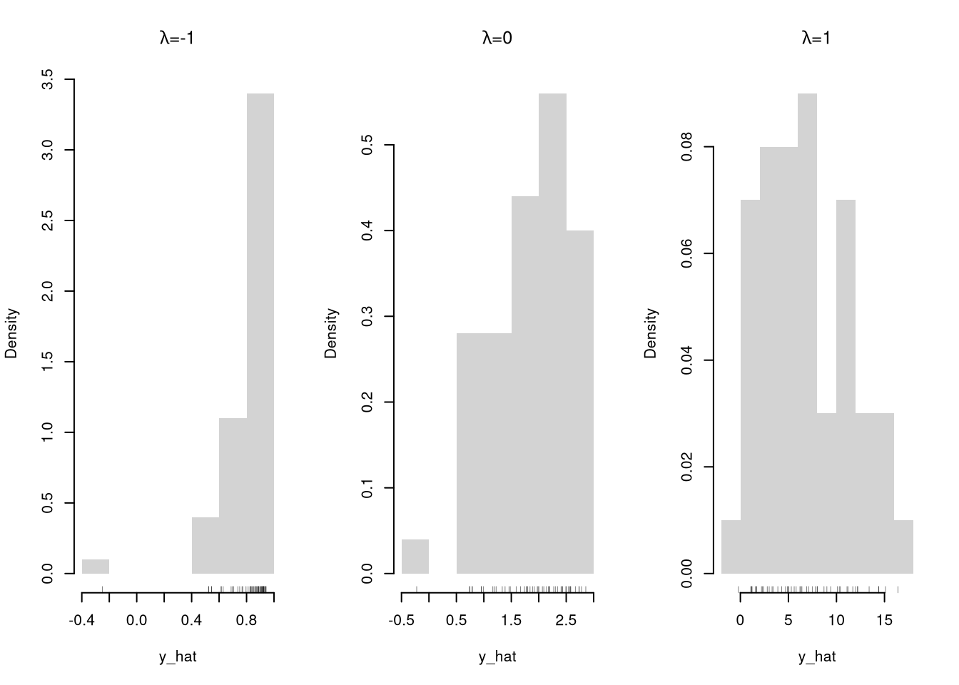
The Box–Cox Transform nests many cases used by statisticians. For \(x>0\) and parameter \(\lambda\), \[
y=\begin{cases}
\dfrac{x^\lambda-1}{\lambda}, & \lambda\neq 0,\\
\log\left(x\right) & \lambda=0.
\end{cases}
\] This function is continuous over \(\lambda\).
Code
# Box–Cox transform and inverse
bc_transform <- function(x_hat, lambda) {
  if (any(x_hat <= 0)) stop('Box-Cox requires x > 0')
  if (abs(lambda) < 1e-8) log(x_hat) else (x_hat^lambda - 1)/lambda
}
bc_inverse <- function(t, lambda) {
  if (abs(lambda) < 1e-8) exp(t) else (lambda*t + 1)^(1/lambda)
}

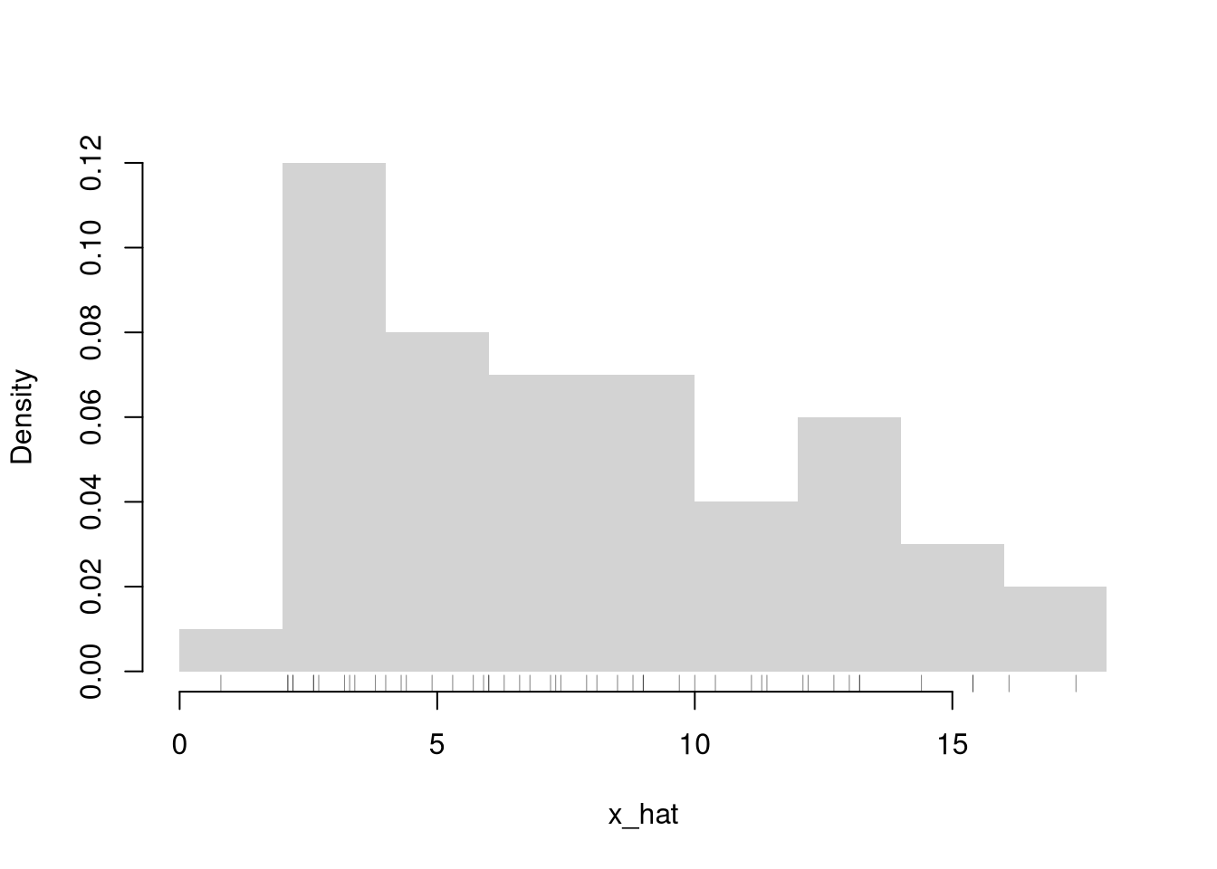
hist(x_hat, main=NA, border=NA, freq=FALSE)
rug(x_hat, col=grey(0, .5))
Code
par(mfrow=c(1, 3))
for(lambda in c(-1, 0, 1)){
    y_hat <- bc_transform(x_hat, lambda)
    hist(y_hat,
        main=NA,
        border=NA, freq=FALSE)
    rug(y_hat, col=grey(0, .5))
    title(bquote(paste(lambda, '=', .(lambda))), font.main=1)
}
Be careful about transforming your data, as the interpretation can be harder.
The mean of transformed data is not equivalent to transforming the mean, for example, which is one reason why you want to first summarize your data before transforming it.
Jensen’s inequality
We can actually say more about how the mean of transformed data is not equivalent to transforming the mean, which we saw for log wages in LOTUS. To do that, we define two types of functions:
- Concave functions curve inwards, like the inside of a cave.
- Convex functions curve outward, the opposite of concave.
Let \(\hat{y}_{i}=g( \hat{x}_{i})\), and denote the mean as \(\hat{m}_{Y}\).
If \(g\) is a concave function, then \(g( \hat{m}_{X} ) \geq \hat{m}_{Y}\). The square root and the log are both concave. Every murder rate is positive, so we can take logs of them all.
Code
# Concave: mean of the transform vs transform of the mean
mean( sqrt(x_hat) )
## [1] 2.671292
sqrt( mean(x_hat) )
## [1] 2.790699

mean( log(x_hat) )
## [1] 1.860618
log( mean(x_hat) )
## [1] 2.052584
Here are some examples.
Code
# Continuous Example 1
x0_hat <- c(0.5, 1.123, 2.987, 3.654)
mean( sqrt(x0_hat) )
## [1] 1.351665
sqrt( mean(x0_hat) )
## [1] 1.437359

# Continuous Example 2
mean( log(x0_hat) )
## [1] 0.4532371
log( mean(x0_hat) )
## [1] 0.7256144
Code
## Discrete Example
x  <- c(1, 2, 3)
px <- c(0.2, 0.5, 0.3)
population_mean_x <- sum(x * px)
population_mean_x
## [1] 2.1

g  <- sqrt
g(population_mean_x)
## [1] 1.449138

population_mean_y <- sum(g(x) * px)
population_mean_y
## [1] 1.426722
If \(g\) is a convex function, then the inequality reverses: \(g( \hat{m}_{X}) \leq \hat{m}_{Y}\). The square \(g(x)=x^2\) is convex.
Code
# Convex: mean of the transform vs transform of the mean
mean( x_hat^2 )
## [1] 79.244
mean( x_hat )^2
## [1] 60.65294
The exponential is also convex. Here it is with three small numbers.
Code
x0_hat <- c(1, 2, 3)
mean( exp(x0_hat) )
## [1] 10.06429
exp( mean(x0_hat) )
## [1] 7.389056
Drawing Samples
To generate a random variable from known distributions, you can use some type of physical machine. E.g., you can roll a fair die to generate Discrete Uniform data or you can roll weighted die to generate Categorical data.
There are also several ways to computationally generate random variables from a probability distribution. Perhaps the most common one is inverse sampling. To generate a random variable using inverse sampling, first sample \(p\) from a uniform distribution and then find the associated quantile via the quantile function \(\hat{F}^{-1}(p)\).
Empirically
You can generate a random variable from a known empirical distribution. Inverse sampling randomly selects observations from the dataset with equal probabilities. To implement this, we
- order the data and associate each observation with an ECDF value
- draw \(p~\text{in}~[0,1]\) as a uniform random variable
- find the associated quantile via the ECDF
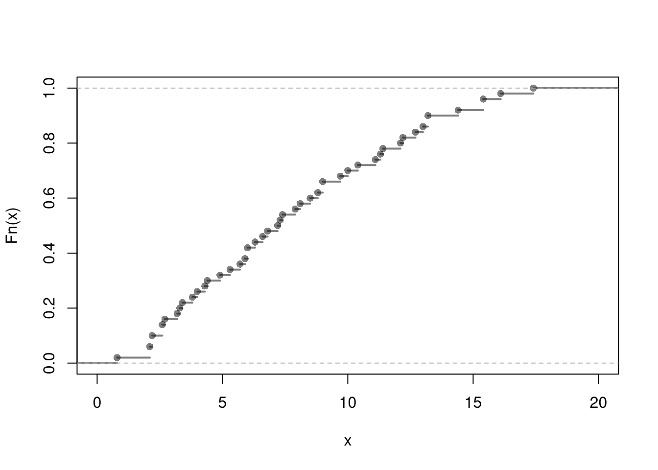
Here is an example of generating random murder rates for US states.
Code
# Empirical Distribution
F_hat <- ecdf(x_hat)
plot(F_hat, lwd=2, xlim=c(0, 20),
    pch=16, col=grey(0, .5), main=NA)
Code
# Generating random variables via inverse ECDF
p <- runif(3000) ## Multiple Draws
x_sim <- quantile(F_hat, p, type=1)
x_sim[c(1, 2, 3)]
## 26.55086631% 37.21238996% 57.28533634%
##          4.3          5.9          8.1

## Can also do directly from the data
x_sim <- quantile(x_hat, p, type=1)
x_sim[c(1, 2, 3)]
## 26.55086631% 37.21238996% 57.28533634%
##          4.3          5.9          8.1
Every draw is one of the observed murder rates, since the ECDF only jumps at the data.
Theoretically
If you know the distribution function that generates the data, then you can derive the quantile function and do inverse sampling. That is how computers generate random data from a distribution.
Code
# 4 random data points from 3 different distributions
runif(4)
## [1] 0.8023495 0.4794952 0.1774016 0.3971333
rexp(4)
## [1] 0.62845399 0.12015702 0.41008008 0.09420932
rnorm(4)
## [1]  0.8917676  1.3292082 -0.1034661  0.6150646
Here is an in-depth example of the Dagum distribution. The distribution function is \(F(x)=(1+(x/b)^{-a})^{-c}\). For a given probability \(p\), we can then solve for the quantile as \[F^{-1}(p)=\frac{ b p^{\frac{1}{ac}} }{(1-p^{1/c})^{1/a}}\] After which, we sample \(p\) from a uniform distribution and then find the associated quantile.
Code
# Theoretical Quantile Function (from VGAM::qdagum)
qdagum <- function(p, scale.b=1, shape1.a, shape2.c) {
  # Quantile function (theoretically derived from the CDF)
  ans <- scale.b * (expm1(-log(p) / shape2.c))^(-1 / shape1.a)
  # Special known cases
  ans[p == 0] <- 0
  ans[p == 1] <- Inf
  # Safety Checks
  ans[p < 0] <- NaN
  ans[p > 1] <- NaN
  if(scale.b <= 0 | shape1.a <= 0 | shape2.c <= 0){ ans <- ans*NaN }
  # Return
  return(ans)
}

# Generate Random Variables (VGAM::rdagum)
rdagum <-function(n, scale.b=1, shape1.a, shape2.c){
    p <- runif(n) # generate random probabilities
    x_sim <- qdagum(p, scale.b=scale.b, shape1.a=shape1.a, shape2.c=shape2.c) #find the inverses
    return(x_sim)
}

# Example
x_sim <- rdagum(3000, 1, 3, 1)
x_sim[c(1, 2, 3)]
## [1] 0.3340868 0.4930646 0.8692034
Exercises
Comment the script you wrote for this chapter, then restart R and check that it runs from a clean session, then check the script with AI as explained in Working with AI. Write three sentences from memory on the main statistical idea of this chapter, and ask the assistant what is wrong, vague, or missing. Finish with your own questions about whatever you found hardest.
Using the dataset \(\{3, 3.1, 0.02\}\) and half-width \(h=1/2\), compute the uniform kernel density \(\hat{f}_{U}(x)\) by hand at \(x=0\), \(x=3\), and \(x=5\). That is, for each \(x\) count the observations within \(h\) of \(x\) and divide by \(n \cdot 2h\). Then write a short R function that does the same count and verify your three answers.
Load USArrests in R and extract the Assault variable. Compute mean(log(x_hat)) and log(mean(x_hat)). Which is larger, and which case of Jensen’s inequality does this illustrate? Then apply the Box–Cox transform with \(\lambda~\text{in}~\{-1, 0, 1/2, 1\}\) using bc_transform from this chapter, and plot the four histograms side by side. Which \(\lambda\) gives the most symmetric histogram?
The exponential distribution with rate \(\lambda\) has distribution function \(F(x)=1-e^{-\lambda x}\) for \(x \geq 0\). Solve for the quantile function \(F^{-1}(p)\) by hand. Write an R function that draws \(n\) values of \(p\) from a uniform distribution and returns \(F^{-1}(p)\), then generate \(5000\) draws with \(\lambda=2\). Plot a histogram of your draws with freq=FALSE and overlay dexp(x_hat, rate=2) to check that they match.
Recall
This chapter collected three tools that extend the univariate toolkit: the kernel density, which smooths a histogram by averaging a weight function centered on each observation with half-width \(h\); data transformations such as the log and the Box–Cox family, together with Jensen’s inequality on how the mean of transformed data compares to the transformed mean; and inverse sampling, which generates random draws by feeding uniform probabilities through a quantile function. The running three-point dataset \(\{3, 3.1, 0.02\}\) pins the first of these down: the uniform kernel density at \(x=3\) with half-width \(h=1/2\) equals \(2/3\), because two points fall inside the interval \([2.5, 3.5]\) and \(2/(3 \times 1)=2/3\). For the second, mean(sqrt(x_hat)) is never larger than sqrt(mean(x_hat)) because the square root is concave, and the inequality flips for a convex function like the exponential.