We now compare two groups: how the distribution of one variable changes across the categories of another. We begin with discrete data and then turn to continuous data. In both cases, a cardinal outcome \(\hat{y}_{i}\) is split into groups by a factor \(\hat{x}_{i}\).
This chapter asks three questions.
- How does \(\hat{y}\) differ across groups?
- Conditional mean and conditional quantile: these compute the mean and the quantiles of \(\hat{y}\) inside each subgroup.
- Difference statistic: this is a new statistic, \(\hat{d}=\hat{g}_{1}-\hat{g}_{2}\), the gap in a statistic such as the mean or the median.
- Do the whole distributions differ?
- KS and CVM statistics: these are new statistics that summarize the gaps between two ECDFs.
- How sure are we?
- Bootstrap confidence interval: this resamples each group separately and tests the difference by inverting a CI.
- Permutation test: this is a new way to impose the null, by reshuffling the group labels.
Discrete Data
When both variables are factors, a natural way to summarize their association is to look at how the average of one (treated as cardinal) changes across categories of the other. When its categories are ordered, we can also look at how its quantiles change.
The conditional mean \(\hat{m}_{Y}(x)\) is the average value of \(\hat{y}_{i}\) inside the subgroup where \(\hat{x}_{i}=x\): \[\hat{m}_{Y}(x)=\sum_{y} y\,\hat{p}(y\mid x).\]
Comparing \(\hat{m}_{Y}(x)\) across values of \(x\) is useful as the simplest summary of association between a cardinal outcome and a factor. One number per subgroup shows whether \(\hat{y}\) tends to be higher in one category. The calculation breaks into two steps: column-by-column, compute the conditional distribution \(\hat{p}(y\mid x)\), then take its weighted average using the values of \(y\).
For example, the code below treats a discrete \(\hat{y}\) as cardinal and compares it across the categories of \(\hat{x}\). We first split \(\hat{y}\) into one group per category, and then average within each group.
Code
## MAIN EXAMPLE
# Lab data: 3294 US workers from the Ecdat package
# school is years of schooling, treated here as cardinal
# sex is a factor with levels female and male
data(Wages1, package='Ecdat')
# Years of schooling within each sex
D_female <- Wages1[, 'sex'] == 'female'
y1_hat <- Wages1[D_female, 'school']
y2_hat <- Wages1[!D_female, 'school']

# Conditional mean of schooling within each sex
m1_hat <- mean(y1_hat)
m2_hat <- mean(y2_hat)
c(m1_hat=m1_hat, m2_hat=m2_hat)
##   m1_hat   m2_hat
## 11.83748 11.44232
# Women in this sample average about 11.8 years and men about 11.4 years.
Alternatively, aggregate computes the conditional mean for every group at once. To see the two steps in the definition, we first compute the conditional distribution of \(\hat{y}\) within each category of \(\hat{x}\), so that each column sums to 1. We then take the weighted average of the values of \(y\) within each column.
Code
# Mean years of school by sex
aggregate(school ~ sex, Wages1, mean)
##      sex   school
## 1 female 11.83748
## 2   male 11.44232

## Breakdown
# Counts of years of schooling (rows) by sex (columns)
school_sex <- table(Wages1[, 'school'], Wages1[, 'sex'])

# Conditional distribution p(y|x): each column sums to 1
p_school_sex <- prop.table(school_sex, 2)
round(p_school_sex, 3)
##
##      female  male
##   3   0.000 0.001
##   4   0.000 0.001
##   5   0.001 0.002
##   6   0.002 0.006
##   7   0.005 0.009
##   8   0.014 0.037
##   9   0.038 0.059
##   10  0.106 0.135
##   11  0.196 0.205
##   12  0.379 0.344
##   13  0.120 0.087
##   14  0.089 0.072
##   15  0.043 0.038
##   16  0.007 0.003
# Men are more common at 10 years or fewer.
# Women are more common at 12 years or more.

# Conditional mean of schooling within each sex
school_values <- as.numeric(rownames(p_school_sex))
m_school_sex <- colSums(school_values * p_school_sex)
m_school_sex
##   female     male
## 11.83748 11.44232
Suppose our data is given in the table shown below.
Counts of \(y\) by \(x\)
| \(y=1\) |
\(12\) |
\(8\) |
| \(y=2\) |
\(18\) |
\(6\) |
| \(y=3\) |
\(10\) |
\(16\) |
First, we compute conditional probabilities to examine how the distribution changes.
Conditional Proportions of \(y\) Given \(x\)
| \(y=1\) |
\(12/40\) |
\(8/30\) |
| \(y=2\) |
\(18/40\) |
\(6/30\) |
| \(y=3\) |
\(10/40\) |
\(16/30\) |
|
\(40/40\) |
\(30/30\) |
Second, we apply the conditional-mean formula column by column: \[\begin{aligned}
\hat{m}_{Y}(x=0) &= 1 \frac{12}{40} + 2 \frac{18}{40} + 3 \frac{10}{40} = \frac{12+36+30}{40} = \frac{78}{40} \\
\hat{m}_{Y}(x=1) &= 1 \frac{8}{30} + 2 \frac{6}{30} + 3 \frac{16}{30} = \frac{8+12+48}{30} = \frac{68}{30}
\end{aligned}\] Notice that \(\hat{m}_{Y}(x=0) < \hat{m}_{Y}(x=1)\), which shows that the mean value of \(\hat{y}\) is higher when \(\hat{x}\) is higher. I.e., there is a positive association.
We can also compare conditional medians by adding up the conditional proportions down each column. When \(x=0\), the running total is \(12/40\) at \(y=1\) and \(30/40\) at \(y=2\), so \(\hat{F}_{Y}^{-1}(0.5 \mid x=0) = 2\). When \(x=1\), the running total is \(8/30\) at \(y=1\), \(14/30\) at \(y=2\), and \(30/30\) at \(y=3\), so \(\hat{F}_{Y}^{-1}(0.5 \mid x=1) = 3\). The median value of \(\hat{y}\) is also higher when \(\hat{x}\) is higher.
We can compute the mean \(\hat{m}_{Y}\) using the marginal distributions, as already shown in the last chapter. To compute the mean, \(\hat{m}_{Y}\), we first compute the joint distribution by dividing each cell with \(12+8+18+6+10+16 = 70\) so that all cells sum to 1. We then sum up proportions along each row and column to compute the marginals.
Joint and Marginal Proportions
| \(y=1\) |
\(12/70\) |
\(8/70\) |
\(20/70\) |
| \(y=2\) |
\(18/70\) |
\(6/70\) |
\(24/70\) |
| \(y=3\) |
\(10/70\) |
\(16/70\) |
\(26/70\) |
| Marginal x |
\(40/70\) |
\(30/70\) |
\(70/70\) |
Second, we compute the overall mean using the marginals \[
\hat{m}_{Y} = 1 \frac{20}{70} + 2 \frac{24}{70} + 3 \frac{26}{70} = \frac{20 + 48 + 78}{70} = {146/70}
\]
Third, we compare \(\hat{m}_{Y}\) to the conditional means from the Must Know box. The overall mean is a weighted average of the two conditional means, where each weight is the marginal proportion \(\hat{p}(x)\): \[\begin{aligned}
\hat{m}_{Y} &= \hat{p}(x=0) \hat{m}_{Y}(x=0) + \hat{p}(x=1) \hat{m}_{Y}(x=1) \\
&= \frac{40}{70} \frac{78}{40} + \frac{30}{70} \frac{68}{30} = \frac{78 + 68}{70} = \frac{146}{70}
\end{aligned}\] A weighted average always lies between the values being averaged, so \(\hat{m}_{Y}(x=0) < \hat{m}_{Y} < \hat{m}_{Y}(x=1)\). In numbers, \(78/40 = 1.95\), \(146/70 \approx 2.09\), and \(68/30 \approx 2.27\).
The conditional mean summarizes each subgroup with one number, but we can also ask where the lower, middle, and upper parts of each subgroup lie.
The conditional quantile is the \(p\)th quantile of \(\hat{y}_{i}\) inside the subgroup where \(\hat{x}_{i}=x\). It inverts the conditional ECDF and is written \(\hat{F}_{Y}^{-1}(p \mid x)\). For discrete \(\hat{y}\), \(\hat{F}_{Y}^{-1}(p \mid x)\) is the smallest \(y\) where \(\hat{F}_{Y}(y \mid x) \geq p\).
Conditional quantiles are useful when \(\hat{y}\) is ordered but not cardinal: unlike the conditional mean, they only use the ordering of the categories, as with ordered factors. In R, quantile with type=1 inverts the ECDF within each group, so it returns an observed value.
Code
## MAIN EXAMPLE
# Conditional medians within each sex
med1_hat <- median(y1_hat)
med2_hat <- median(y2_hat)
c(med1_hat=med1_hat, med2_hat=med2_hat)
## med1_hat med2_hat
##       12       12
# The medians are both 12 years.
# That is because over a third of each group stopped at exactly 12 years.

# Conditional quartiles within each sex
q1_hat <- quantile(y1_hat, probs=c(.25, .5, .75), type=1)
q2_hat <- quantile(y2_hat, probs=c(.25, .5, .75), type=1)
rbind(q1_hat, q2_hat)
##        25% 50% 75%
## q1_hat  11  12  13
## q2_hat  10  12  12
# The quartiles still show a difference.
# The middle half of women have between 11 and 13 years.
# The middle half of men have between 10 and 12 years.
With lumpy discrete data, a single median can hide a difference that several quantiles reveal.
Alternatively, aggregate computes the conditional quantiles for every group at once. To see where these quantiles come from, cumsum down each column of the conditional distribution gives \(\hat{F}_{Y}(y \mid x)\) for each group. Each quartile is the first row where its column reaches \(p\).
Code
# Conditional Quantiles
aggregate(school ~ sex, Wages1, median)
##      sex school
## 1 female     12
## 2   male     12
aggregate(school ~ sex, Wages1, quantile, probs=c(.25, .5, .75), type=1)
##      sex school.25% school.50% school.75%
## 1 female         11         12         13
## 2   male         10         12         12

## Breakdown
# Conditional ECDF within each sex: cumulative proportions down each column
F_school_sex <- apply(p_school_sex, 2, cumsum)
round(F_school_sex, 3)
##
##      female  male
##   3   0.000 0.001
##   4   0.000 0.002
##   5   0.001 0.004
##   6   0.003 0.010
##   7   0.008 0.020
##   8   0.022 0.057
##   9   0.060 0.115
##   10  0.166 0.250
##   11  0.361 0.456
##   12  0.740 0.800
##   13  0.860 0.887
##   14  0.950 0.959
##   15  0.993 0.997
##   16  1.000 1.000
Continuous Data
Consider a mixed dataset where \(\hat{y}_{i}\) is a continuous cardinal variable and \(\hat{x}_{i}\) is a factor variable (typically unordered). For such “grouped data”, we analyze associations via group comparisons. The basic idea is best seen in a comparison of two samples, which corresponds to an \(\hat{x}_{i}\) with two categories. For example, we might compare the heights of men and women in Canada or the homicide rates in two different American states.
To compare two groups, we start by making a histogram for each.
Code
## MAIN EXAMPLE
# Compare wages for people who did and did not complete a degree
# Workers with 12 or 16 years of schooling, and which of them are high school only
xy_hat <- Wages1[Wages1[, 'school'] %in% c(12, 16), c('school', 'wage')]
D_hs <- xy_hat[, 'school'] == 12

# Hourly wages within each level of schooling
y1_hat <- xy_hat[D_hs, 'wage'] # high school only
y2_hat <- xy_hat[!D_hs, 'wage'] # university graduates

# Initial summary figure: two overlaid histograms on a common grid
bks <- seq(0, 34, by=1)             # shared bin edges
dlim <- c(0, .2)                    # shared y limit
cols <- c(rgb(.8, 0, 0, .5), rgb(0, 0, .8, .5)) # semi-transparent fill

hist(y1_hat, breaks=bks, ylim=dlim,
     col=cols[1], xlab='Wages',
     freq=FALSE, border=NA, main=NA)
rug(y1_hat, col=cols[1])
hist(y2_hat, breaks=bks, ylim=dlim,
     col=cols[2],
     freq=FALSE, border=NA, add=TRUE)
rug(y2_hat, col=cols[2])
legend('topright',
       col=cols, pch=15,
       legend=c('12 Years (High School)', '16 Years (University)'),
       title='School Completed')
The histogram may show several differences between groups or none at all. In general, we test whether the difference in some statistic \(\hat{g}\) equals \(0\). As in LOTUS and Data Transformations, \(g\) denotes a function, but here \(\hat{g}\) is a function of a group’s whole sample rather than of a single observation. Often, the first statistic we investigate for hypothesis testing is the mean, \(\hat{m}\).
The difference statistic is the sample-statistic in group 1 minus the sample-statistic in group 2: \[\hat{d} = \hat{g}_{1} - \hat{g}_{2},\] where \(\hat{g}_{1}\) and \(\hat{g}_{2}\) are the statistic computed from the group 1 data and the group 2 data, such as the means \(\hat{m}_{1}\) and \(\hat{m}_{2}\) or the medians \(\tilde{m}_{1}\) and \(\tilde{m}_{2}\). A positive value says the statistic is higher in group 1, zero means no difference between groups, and a negative value says the statistic is higher in group 2.
Mean Differences
The mean difference is useful for summarizing how different two groups are on average. It is on the same scale as the outcome. Its null hypothesis is no difference in population means, \(H_{0}: \mathbb{E}[Y_{i1}]=\mathbb{E}[Y_{i2}]\). We can test that hypothesis by inverting a confidence interval. The code below computes \(\hat{m}_{1}\) and \(\hat{m}_{2}\) and reports \(\hat{d}\). Is the gap bigger than we would expect from sampling noise? To answer that, we resample each group separately and recompute \(\hat{d}\) each time.
Code
## MAIN EXAMPLE
# Difference between means
m1_hat <- mean(y1_hat)
m2_hat <- mean(y2_hat)
d_hat <- m1_hat - m2_hat
round(c(m1_hat=m1_hat, m2_hat=m2_hat, d_hat=d_hat), 2)
## m1_hat m2_hat  d_hat
##   5.67   7.54  -1.87
# The university group has the higher mean wage, so d_hat is negative.

# Bootstrap Distribution
bootstrap_diff <- rep(NA, 9999)
for(b in seq(bootstrap_diff) ){
    # keep each worker's group fixed and resample wages within each group
    y1_boot <- sample(xy_hat[D_hs, 'wage'], replace=TRUE)
    y2_boot <- sample(xy_hat[!D_hs, 'wage'], replace=TRUE)
    m1_b_hat <- mean(y1_boot)
    m2_b_hat <- mean(y2_boot)
    d_b <- m1_b_hat - m2_b_hat
    bootstrap_diff[b] <- d_b
}
hist(bootstrap_diff, breaks=50,
    border=NA, freq=FALSE,
    main=NA, xlab='Difference in Means')
title('Bootstrapped Difference in Means', font.main=1)

# 2-Sided Test via Confidence Interval
boot_ci <- quantile(bootstrap_diff, probs=c(.025, .975))
abline(v=boot_ci, col=rgb(0, 0, 0, .8), lwd=2)
abline(v=0, col=rgb(0, 0, 1, .8), lty=2)
Such tests make purely statistical statements that only speak to how frequently differences are generated by random chance. They do not say why there are any differences or how large they are. Even on purely statistical grounds, however, we would want to be cautious about making data-driven decisions when
- the significance level is somewhat arbitrary (what if we reject at the \(5\%\) level but not \(10\%\) level?)
- the test statistic is somewhat arbitrary (what if we reject for means but not medians?)
- there are multiple differences
For such reasons, applied statisticians consider many statistics.
Quantile Differences
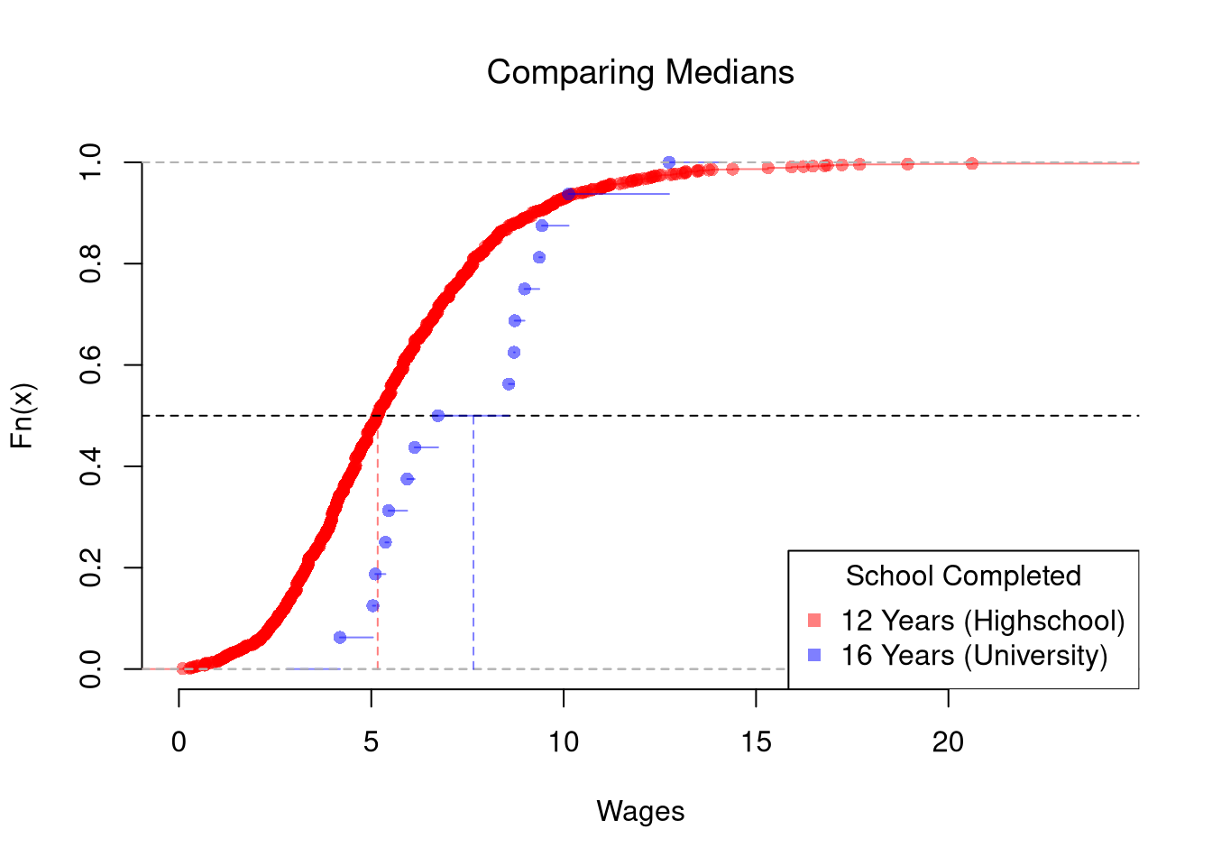
The above procedure generalizes from differences in means to differences in medians. To start, we plot the ECDF’s for both groups.
Code
# Quantile Comparison

## Distribution 1
F1_hat <- ecdf(y1_hat)
plot(F1_hat, col=cols[1],
     pch=16, xlab='Wages', xlim=c(0, 24),
     main=NA, bty='n')
title('Comparing Medians', font.main=1)
## Median 1
med1_hat <- median(y1_hat) # equivalently, quantile(F1_hat, probs=0.5)
segments(med1_hat, 0, med1_hat, 0.5, col=cols[1], lty=2)
abline(h=0.5, col=grey(.5), lty=3)

## Distribution 2
F2_hat <- ecdf(y2_hat)
plot(F2_hat, add=TRUE, col=cols[2], pch=16)
## Median 2
med2_hat <- median(y2_hat) # equivalently, quantile(F2_hat, probs=0.5)
segments(med2_hat, 0, med2_hat, 0.5, col=cols[2], lty=2)

## Legend
legend('bottomright',
       col=cols, pch=15,
       legend=c('12 Years (High School)', '16 Years (University)'),
       title='School Completed')
Code
# Bootstrap Distribution Function
boot_quant <- function(y_hat, D_group, n_boot=9999, probs=0.5, ...){
    bootstrap_diff <- rep(NA, n_boot)
    for(b in seq(bootstrap_diff)){
        y1_boot <- sample(y_hat[D_group], replace=TRUE)
        y2_boot <- sample(y_hat[!D_group], replace=TRUE)
        q1_b <- quantile(y1_boot, probs=probs, ...)
        q2_b <- quantile(y2_boot, probs=probs, ...)
        d_b <- q1_b - q2_b
        bootstrap_diff[b] <- d_b
    }
    return(bootstrap_diff)
}

# 2-Sided Test for Median Differences
d_med <- med1_hat - med2_hat
d_med
## [1] -2.489273
boot_d <- boot_quant(xy_hat[, 'wage'], D_hs, n_boot=9999, probs=0.5)
hist(boot_d, breaks=50, border=NA, freq=FALSE,
    main=NA, xlab='Difference in Medians')
title('Bootstrap Difference in Medians', font.main=1)
abline(v=quantile(boot_d, probs=c(.025, .975)), col=rgb(0, 0, 0, .8), lwd=2)
abline(v=0, col=rgb(0, 0, 1, .8), lty=2)
Changing probs in boot_quant tests other quantiles, such as the quartiles. Note that bootstrap tests can perform poorly with highly unequal variances or skewed data. To see this yourself, make a simulation with skewed data and unequal variances.
Other Statistics
In principle, we can also examine whether there are differences in spread (sd or IQR) or shape (skew or kurtosis). We use the same hypothesis testing procedure as above.
Here is an example to look at differences in “spread”
Code
boot_fun <- function( fun, n_boot=9999, ...){
    bootstrap_diff <- rep(NA, n_boot)
    for(b in seq(bootstrap_diff)){
        y1_boot <- sample(xy_hat[D_hs, 'wage'], replace=TRUE)
        y2_boot <- sample(xy_hat[!D_hs, 'wage'], replace=TRUE)
        f1_b <- fun(y1_boot, ...)
        f2_b <- fun(y2_boot, ...)
        d_b <- f1_b - f2_b
        bootstrap_diff[b] <- d_b
    }
    return(bootstrap_diff)
}

# 2-Sided Test for SD Differences
d_sd <- sd(y1_hat) - sd(y2_hat)
d_sd
boot_d <- boot_fun(sd)
hist(boot_d, breaks=50, border=NA, freq=FALSE,
    main=NA, xlab='Difference in Standard Deviations')
title('Bootstrap Difference in Standard Deviations', font.main=1)
abline(v=quantile(boot_d, probs=c(.025, .975)), col=rgb(0, 0, 0, .8), lwd=2)
abline(v=0, col=rgb(0, 0, 1, .8), lty=2)

# Try any function!
# boot_fun( function(xs) { IQR(xs)/median(xs) } )
Distributional Comparisons
We can also examine whether there are any differences between the entire distributions. We typically start by plotting the two ECDF’s, and then calculate a statistic for hypothesis testing. A quantile-quantile plot is another way to compare the two distributions visually.
KS and CVM Statistics
To go from a picture of two distributions to a single-number summary of how different they are, we measure the gap between their ECDFs.
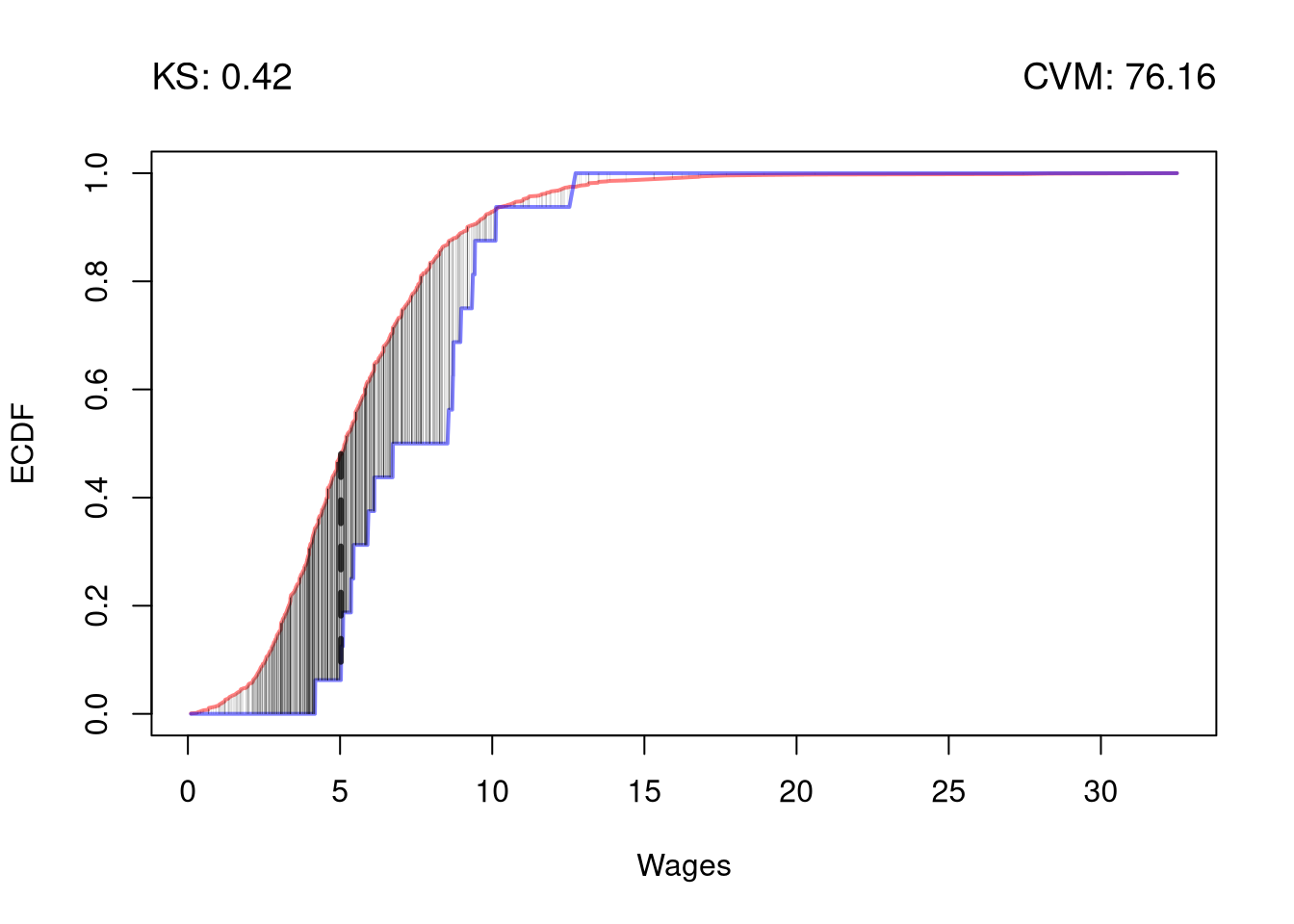
The Kolmogorov-Smirnov statistic \(\hat{\text{KS}}\) (Kolmogorov 1933; Smirnov 1948) summarizes the difference between two ECDFs by their single biggest vertical gap, evaluated over the pooled sample \(y~\text{in}~\{\hat{y}_{i1}\} \cup \{\hat{y}_{i2}\}\): \[\hat{\text{KS}} = \max_{y} |\hat{F}_{1}(y)- \hat{F}_{2}(y)|^{p}.\]
The Cramer-von Mises statistic \(\hat{\text{CVM}}\) (Cramér 1928; von Mises 1928; Anderson 1962) instead sums the vertical gaps at every pooled sample point: \[\hat{\text{CVM}} = \sum_{y} | \hat{F}_{1}(y)- \hat{F}_{2}(y)|^{p}.\]
The integer \(p\) is typically \(1\) for \(\hat{\text{KS}}\) and \(2\) for \(\hat{\text{CVM}}\).
\(\hat{\text{KS}}\) is useful when we expect distributions to differ by a shift: the gap piles up at one location and the max catches it. The cost is that \(\hat{\text{KS}}\) uses only the single largest gap, so it can miss many small differences spread across the support. \(\hat{\text{CVM}}\) is useful for accumulated small differences spread across the support, since every pooled sample point contributes to the sum.
Code
## MAIN EXAMPLE
# KS and CVM statistics for any two-group split
ks_cvm <- function(y1_hat, y2_hat){
    y_values <- sort(c(y1_hat, y2_hat)) # pooled sample points
    F1_vals <- ecdf(y1_hat)(y_values)
    F2_vals <- ecdf(y2_hat)(y_values)
    gap <- abs(F1_vals - F2_vals)
    # KS: largest vertical gap (p=1); CVM: summed squared gaps (p=2)
    return(c(KS=max(gap), CVM=sum(gap^2)))
}
stat_obs <- ks_cvm(y1_hat, y2_hat)
round(stat_obs, 2)
##    KS   CVM
##  0.42 76.16
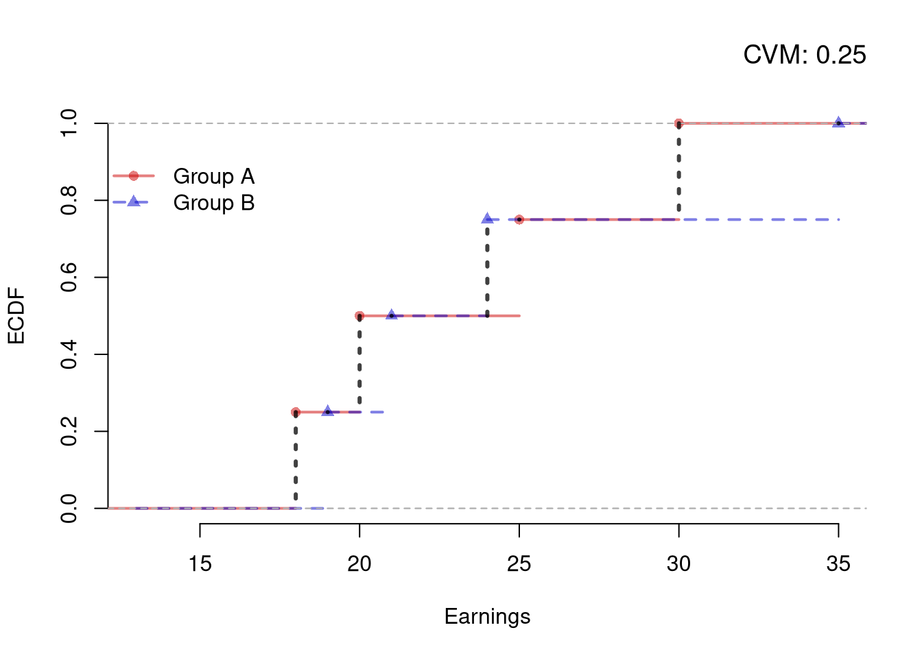
Suppose there are two groups of summer workers, with data on the earnings of each individual. In thousands of Canadian Dollars, specifically, Group \(A\) has earnings \(\{18,20,25,30\}\) and group \(B\) has earnings \(\{19,21,24,35\}\).
We can compute the CVM and KS statistics for further statistical testing. Start by drawing the ECDF’s.
Code
# Earnings of each group, in thousands of Canadian Dollars
yA0_hat <- c(18, 20, 25, 30)
yB0_hat <- c(19, 21, 24, 35)
FA_hat <- ecdf(yA0_hat)
FB_hat <- ecdf(yB0_hat)

# ECDFs as step functions; shape and line type also mark the group
plot(FA_hat, col=cols[1], pch=16, lwd=2,
    xlab='Earnings', ylab='ECDF',
    main=NA, bty='n')
plot(FB_hat, add=TRUE, col=cols[2], pch=17, lty=2, lwd=2)

# Vertical gaps at the 8 pooled values, one per row of the table below
x_values <- sort(c(yA0_hat, yB0_hat))
segments(x_values, FA_hat(x_values), x_values, FB_hat(x_values),
    lwd=3, col=grey(0, .75), lty=3)
cvm0_hat <- sum((FA_hat(x_values) - FB_hat(x_values))^2)
title(paste0('CVM: ', cvm0_hat), adj=1, font.main=1)

legend('topleft', bty='n', inset=c(0, .1),
    col=cols, pch=c(16, 17), lty=c(1, 2), lwd=2,
    legend=c('Group A', 'Group B'))
Each dotted segment is a gap of \(1/4\), and at the other four pooled values the two ECDFs meet. Then compute \(\hat{F}_{A}(x) - \hat{F}_{B}(x)\) and its square at each of the 8 pooled sorted values:
ECDF Gaps at Each Pooled Value
| 18 |
1/4 |
0 |
1/4 |
1/16 |
| 19 |
1/4 |
1/4 |
0 |
0 |
| 20 |
2/4 |
1/4 |
1/4 |
1/16 |
| 21 |
2/4 |
2/4 |
0 |
0 |
| 24 |
2/4 |
3/4 |
-1/4 |
1/16 |
| 25 |
3/4 |
3/4 |
0 |
0 |
| 30 |
4/4 |
3/4 |
1/4 |
1/16 |
| 35 |
4/4 |
4/4 |
0 |
0 |
\(\text{CVM} = 1/16 + 1/16 + 1/16 + 1/16 = 1/4\).
The KS statistic is the largest absolute value in the \(\hat{F}_{A}-\hat{F}_{B}\) column. \(\text{KS} = \max\{1/4, 0, 1/4, 0, |-1/4|, 0, 1/4, 0\} = 1/4\).
Quantile-Quantile Plots
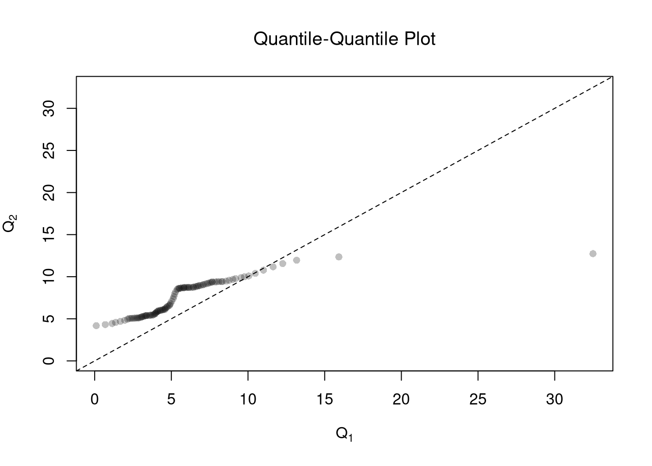
Another useful visualization for two groups is to plot the quantiles against one another: a quantile-quantile plot. I.e., the first data point on the bottom left shows the first quantile for both distributions.
Code
# Percentiles of each group's wages
quants <- seq(0, 1, length.out=101)
Q1 <- quantile(y1_hat, probs=quants)
Q2 <- quantile(y2_hat, probs=quants)

# Compare Quantiles
ry <- range(c(y1_hat, y2_hat))
plot(Q1, Q2, xlim=ry, ylim=ry,
    xlab=expression(Q[1]),
    ylab=expression(Q[2]),
    main=NA,
    pch=16, col=grey(0, .25))
title('Quantile-Quantile Plot', font.main=1)
abline(a=0, b=1, col=rgb(0, 0, 1, .8), lty=2)
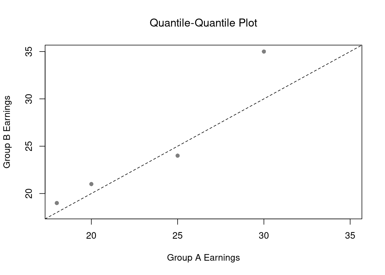
Return to the summer workers from the Must Know above, with group \(A\) earning \(\{18,20,25,30\}\) and group \(B\) earning \(\{19,21,24,35\}\). Compare the two distributions by drawing a QQ plot.
We sort both samples and plot Group \(A\) quantiles (x-axis) against Group \(B\) quantiles (y-axis): \((18,19),\ (20,21),\ (25,24),\ (30,35)\).
Code
# Sorting pairs the k-th smallest earnings in group A with the k-th smallest in group B
ry0 <- range(c(yA0_hat, yB0_hat))
plot(sort(yA0_hat), sort(yB0_hat), xlim=ry0, ylim=ry0,
    xlab='Group A Earnings', ylab='Group B Earnings',
    main=NA, pch=16, col=grey(0, .5))
title('Quantile-Quantile Plot', font.main=1)
abline(a=0, b=1, col=rgb(0, 0, 1, .8), lty=2) # 45 degree line: identical distributions
The 45° reference line indicates identical distributions. Point 1, \((18,19)\), lies above the line, and so do points 2 and 4.
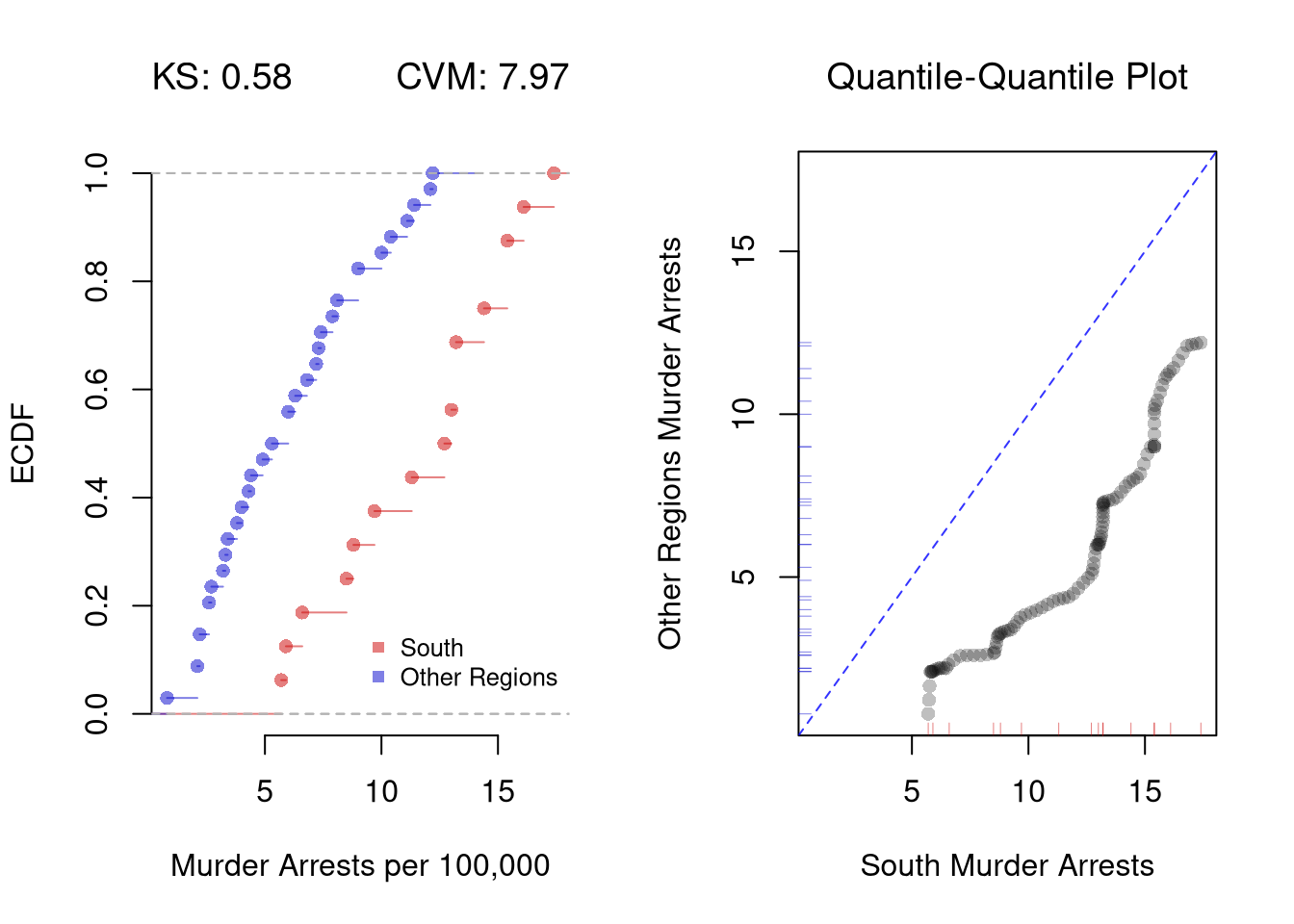
Repeat these comparisons for the \(50\) states in USArrests, with murder arrests split into the South and the other census regions. Compute the KS and CVM statistics, then draw the two ECDFs and a QQ plot. Is the South higher at every percentile?
Code
# 50 US states in 1973, with murder arrests per 100,000 people.
# The built-in state.region lists regions in the same state order as USArrests.
D_south <- state.region == 'South'
murder1_hat <- USArrests[D_south, 'Murder']  # 16 southern states
murder2_hat <- USArrests[!D_south, 'Murder'] # 34 states in other regions

# KS and CVM statistics, with ks_cvm() from above
stat2_obs <- ks_cvm(murder1_hat, murder2_hat)
round(stat2_obs, 2)
##   KS  CVM
## 0.58 7.97
# The two ECDFs are up to 0.58 apart.

par(mfrow=c(1, 2))

# ECDFs on a common axis
ry2 <- range(c(murder1_hat, murder2_hat))
plot(ecdf(murder1_hat), col=cols[1], pch=16, xlim=ry2,
    xlab='Murder Arrests per 100,000', ylab='ECDF',
    main=NA, bty='n')
plot(ecdf(murder2_hat), add=TRUE, col=cols[2], pch=16)
title(paste0('KS: ', round(stat2_obs[['KS']], 2)), adj=0, font.main=1)
title(paste0('CVM: ', round(stat2_obs[['CVM']], 2)), adj=1, font.main=1)
legend('bottomright', bty='n', cex=.8, inset=c(0, .05),
    col=cols, pch=15,
    legend=c('South', 'Other Regions'))

# Percentiles of each group's murder arrests
Q1_murder <- quantile(murder1_hat, probs=quants)
Q2_murder <- quantile(murder2_hat, probs=quants)

# Compare Quantiles
plot(Q1_murder, Q2_murder, xlim=ry2, ylim=ry2,
    xlab='South Murder Arrests', ylab='Other Regions Murder Arrests',
    main=NA,
    pch=16, col=grey(0, .25))
title('Quantile-Quantile Plot', font.main=1)
abline(a=0, b=1, col=rgb(0, 0, 1, .8), lty=2) # 45 degree line: identical distributions
# Raw observations for each group along its own axis
rug(murder1_hat, side=1, col=cols[1])
rug(murder2_hat, side=2, col=cols[2])
Code
# Every percentile is higher in the South, so all the points lie below the line.
# The gap is largest near the median, at about 7.6 arrests per 100,000.
Permutation Tests
The mean and median tests above invert a bootstrap confidence interval. We can also test by “imposing the null”, where it is more common to use \(p\)-values instead of confidence intervals.
A permutation test of “no difference between groups” recomputes the test statistic on many random reshufflings of the group labels. Because each reshuffle keeps the pooled data but breaks the link between label and outcome, the resulting distribution shows what differences look like under the null of no association.
The permutation test (also called a randomization test) is useful when the null hypothesis is “no association”. Reshuffling the labels imposes that null, and we do not need to assume a distributional form. Every reshuffle uses the same pooled data, so the only variability comes from re-splitting the labels. If using a hard decision rule, it is most common to reject the null at the \(5\%\) level when \(p<0.05\) and fail to reject when \(p \geq 0.05\). Alternatively, we can reject when the observed statistic falls outside the middle \(95\%\) of the permutation distribution, as with the null bootstrap in Hypothesis Testing.
Permuting Means
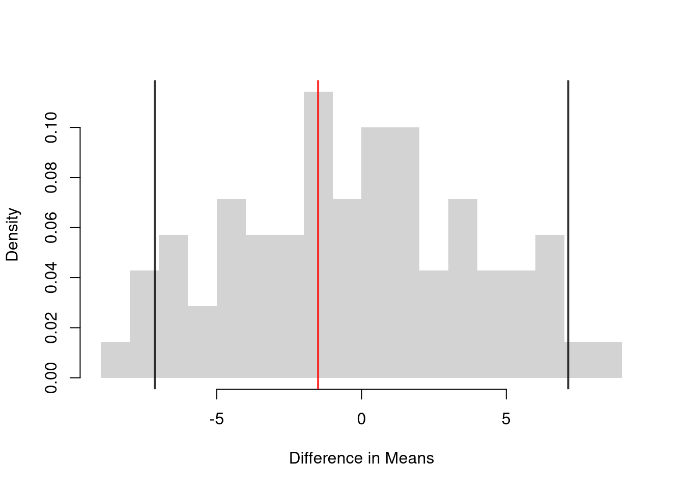
Consider again the two groups of summer workers, with earnings in thousands of Canadian Dollars. Group \(A\) has earnings \(\{18,20,25,30\}\) and group \(B\) has earnings \(\{19,21,24,35\}\). The observed mean difference is \(\hat{d}=23.25-24.75=-1.5\). A permutation keeps the eight pooled values but reassigns which four belong to group \(A\).
Code
# Pooled earnings and group labels (1=A, 2=B)
y0_hat <- c(yA0_hat, yB0_hat) # group A's four earnings, then group B's
g0 <- c(1, 1, 1, 1, 2, 2, 2, 2)
d0_hat <- mean(y0_hat[g0==1]) - mean(y0_hat[g0==2])
d0_hat
## [1] -1.5

# A few reshuffled labels, written out by hand
g0_perm1 <- c(2, 1, 1, 2, 1, 2, 1, 2)
g0_perm2 <- c(1, 2, 2, 1, 1, 2, 1, 2)
g0_perm3 <- c(2, 2, 1, 1, 1, 2, 2, 1)
mean(y0_hat[g0_perm1==1]) - mean(y0_hat[g0_perm1==2])
## [1] -4
mean(y0_hat[g0_perm2==1]) - mean(y0_hat[g0_perm2==2])
## [1] -2.5
mean(y0_hat[g0_perm3==1]) - mean(y0_hat[g0_perm3==2])
## [1] 6.5

# With 8 values there are only choose(8, 4)=70 ways to pick group A
id_A <- combn(8, 4)
d0_perm <- apply(id_A, 2, function(id){
    yA0_perm <- y0_hat[id]
    yB0_perm <- y0_hat[-id]
    mean(yA0_perm) - mean(yB0_perm)
})
hist(d0_perm, breaks=25, border=NA, freq=FALSE,
    main=NA, xlab='Difference in Means')

# 2-Sided Test via the middle 95% of the relabelings
perm0_ci <- quantile(d0_perm, probs=c(.025, .975))
perm0_ci
##    2.5%   97.5%
## -7.1375  7.1375
abline(v=perm0_ci, col=rgb(0, 0, 0, .8), lwd=2)
abline(v=d0_hat, col=rgb(1, 0, 0, .8), lwd=2)
Code
# Two-sided p-value: share of relabelings at least as extreme as observed
mean(abs(d0_perm) >= abs(d0_hat))
## [1] 0.7714286
About \(77\%\) of the \(70\) relabelings produce a gap at least as large as \(1.5\), so this small difference is easy to explain by chance. Likewise, \(\hat{d}=-1.5\) sits well inside the middle \(95\%\) of relabelings, from about \(-7.1\) to \(7.1\).
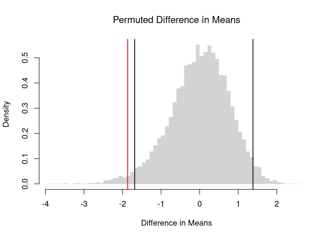
With larger samples, there are far too many relabelings to list, so we draw many of them at random.
Code
## MAIN EXAMPLE
# Permutation Distribution: re-split the pooled wages of the two groups
permute_diff <- rep(NA, 9999)
for(b in seq(permute_diff) ){
    #randomize data
    D_hs0 <- sample(D_hs)
    y1_perm <- xy_hat[D_hs0, 'wage']
    y2_perm <- xy_hat[!D_hs0, 'wage']
    # recompute statistic
    m1_perm_hat <- mean(y1_perm)
    m2_perm_hat <- mean(y2_perm)
    d_b <- m1_perm_hat - m2_perm_hat
    permute_diff[b] <- d_b
}
hist(permute_diff, breaks=50,
    border=NA, freq=FALSE,
    main=NA, xlab='Difference in Means')
title('Permuted Difference in Means', font.main=1)

# 2-Sided Test via the middle 95% of the permutation distribution
perm_ci <- quantile(permute_diff, probs=c(.025, .975))
abline(v=perm_ci, col=rgb(0, 0, 0, .8), lwd=2)
abline(v=d_hat, col=rgb(1, 0, 0, .8), lwd=2)
Code
# Two-sided p-value: share of permutations at least as extreme as observed
p <- mean(abs(permute_diff) >= abs(d_hat))
p
## [1] 0.02060206
Permuting Quantiles
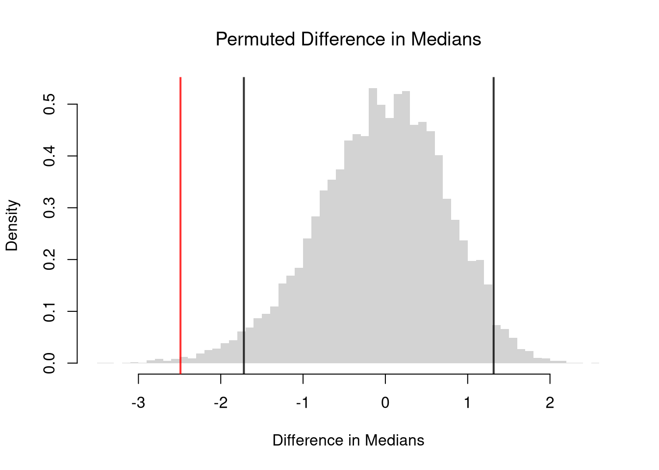
The same reshuffling works for medians: only the statistic that we recompute on each permutation changes. We pool the outcomes of the two groups, randomly pick which of them belong to group 1, and compute the difference in medians.
Code
# Observed difference in medians
d_med <- med1_hat - med2_hat

# Permutation Distribution: same re-split as for means, recomputing medians
permute_med_diff <- rep(NA, 9999)
for(b in seq(permute_med_diff) ){
    D_hs0 <- sample(D_hs)
    y1_perm <- xy_hat[D_hs0, 'wage']
    y2_perm <- xy_hat[!D_hs0, 'wage']
    permute_med_diff[b] <- median(y1_perm) - median(y2_perm)
}
hist(permute_med_diff, breaks=50,
    border=NA, freq=FALSE,
    main=NA, xlab='Difference in Medians')
title('Permuted Difference in Medians', font.main=1)

# 2-Sided Test via the middle 95% of the permutation distribution
perm_med_ci <- quantile(permute_med_diff, probs=c(.025, .975))
abline(v=perm_med_ci, col=rgb(0, 0, 0, .8), lwd=2)
abline(v=d_med, col=rgb(1, 0, 0, .8), lwd=2)
Code
# Two-sided p-value: share of permutations at least as extreme as observed
p_med <- mean(abs(permute_med_diff) >= abs(d_med))
p_med
## [1] 0.00350035
The \(p\)-value is the share of permutations with a median gap at least as large as the observed one. A small \(p\)-value means the observed gap in medians is hard to explain by chance.
Return to the summer workers from the Must Know above, with group \(A\) earning \(\{18,20,25,30\}\) and group \(B\) earning \(\{19,21,24,35\}\). Both groups have the same median, \((20+25)/2 = 22.5\) and \((21+24)/2 = 22.5\), so the observed median difference is \(0\). Every relabeling has a median gap at least as large as \(0\), so the permutation \(p\)-value is \(1\).
Code
# Median difference for all 70 ways to pick group A
d0_med <- median(y0_hat[g0==1]) - median(y0_hat[g0==2])
d0_med_perm <- apply(id_A, 2, function(id){
    yA0_perm <- y0_hat[id]
    yB0_perm <- y0_hat[-id]
    median(yA0_perm) - median(yB0_perm)
})
mean(abs(d0_med_perm) >= abs(d0_med))
## [1] 1
The means differ by \(1.5\), but the medians do not differ at all. A permutation test only looks for differences in the statistic it recomputes, so the choice of statistic matters.
Permuting Distributions
The same reshuffling tests whether the \(\hat{\text{KS}}\) and \(\hat{\text{CVM}}\) statistics from Distributional Comparisons are bigger than chance alone would produce. To impose the null hypothesis of identical distributions, we permute the group labels: each resample keeps the pooled data but randomly re-splits it into two groups of the original sizes. Some permutations produce a statistic at least as large as the observed one. In those cases, random label-shuffling alone created a gap this big. The \(p\)-value is the fraction of such permutations. A small \(p\)-value means the observed gap is hard to explain by chance. Both statistics are never negative, and only large values count against the null. So we use a one-sided interval. We reject at the \(5\%\) level when the observed statistic exceeds the \(95\)th percentile of its permutation distribution.
Code
# ks_cvm() and the observed statistics stat_obs come from Distributional Comparisons

# Permutation null distribution: reshuffle group labels
perm_stats <- matrix(NA, nrow=999, ncol=2,
    dimnames=list(NULL, c('KS', 'CVM')))
for(b in seq(nrow(perm_stats))){
    D_hs0 <- sample(D_hs)
    y1_perm <- xy_hat[D_hs0, 'wage']
    y2_perm <- xy_hat[!D_hs0, 'wage']
    perm_stats[b, ] <- ks_cvm(y1_perm, y2_perm)
}

# Permutation p-values
p_ks  <- mean(perm_stats[, 'KS']  >= stat_obs['KS'])
p_cvm <- mean(perm_stats[, 'CVM'] >= stat_obs['CVM'])

# One-sided critical values: 95th percentile of each permutation distribution
perm_crit <- apply(perm_stats, 2, quantile, probs=.95)
round(c(KS_stat=stat_obs[['KS']], KS_crit=perm_crit[['KS']], KS_pval=p_ks,
    CVM_stat=stat_obs[['CVM']], CVM_crit=perm_crit[['CVM']], CVM_pval=p_cvm), 3)
##  KS_stat  KS_crit  KS_pval CVM_stat CVM_crit CVM_pval
##    0.418    0.330    0.007   76.164   34.893    0.003
Exercises
Comment the script you wrote for this chapter, then restart R and check that it runs from a clean session, then check the script with AI as explained in Working with AI. Write three sentences from memory on the main statistical idea of this chapter, and ask the assistant what is wrong, vague, or missing. Finish with your own questions about whatever you found hardest.
A permutation test shuffles the group labels to build a null distribution, while a bootstrap test resamples with replacement from each group separately. Explain why permutation is appropriate for testing “no difference between groups” and when you might prefer the bootstrap instead.
Using the Wages1 data from the Ecdat package, compute the difference in mean wages \(\hat{d} = \hat{m}_{1} - \hat{m}_{2}\) between men and women (the sex variable). Then compute the Kolmogorov-Smirnov statistic \(\hat{\text{KS}}\) between the two wage distributions by hand (i.e., find the maximum absolute difference between the two ECDF’s evaluated at the pooled sorted data).
Using the mtcars dataset, split cars into two groups based on transmission type (am: 0 = automatic, 1 = manual). Write a permutation test with \(B = 9999\) iterations to test whether the difference in mean mpg between automatic and manual cars is statistically different from zero. Report the \(p\)-value.
Recall
This chapter compared two groups by their means, their quantiles, and their whole distributions using \(\hat{\text{KS}}\) and \(\hat{\text{CVM}}\). The main example compared wages in Wages1 for workers with 12 and 16 years of schooling, with permutation tests for \(p\)-values. A small example used summer earnings \(A=\{18,20,25,30\}\) and \(B=\{19,21,24,35\}\). We found \(\hat{d}=-1.5\) by hand, listed all \(70\) relabelings in R for a permutation \(p\)-value of about \(0.77\), and computed \(\hat{\text{CVM}}=1/4\) cell by cell.
Anderson, T. W. 1962.
“On the Distribution of the Two-Sample Cramér-von Mises Criterion.” The Annals of Mathematical Statistics 33 (3): 1148–59.
https://doi.org/10.1214/aoms/1177704477.
Cramér, Harald. 1928.
“On the Composition of Elementary Errors.” Scandinavian Actuarial Journal 1928 (1): 13–74.
https://doi.org/10.1080/03461238.1928.10416862.
Kolmogorov, A. N. 1933.
“Sulla determinazione empirica di una legge di distribuzione.” Giornale dell’Istituto Italiano degli Attuari 4: 83–91.
https://doi.org/10.1007/978-94-011-2260-3_15.
Smirnov, N. 1948.
“Table for Estimating the Goodness of Fit of Empirical Distributions.” The Annals of Mathematical Statistics 19 (2): 279–81.
https://doi.org/10.1214/aoms/1177730256.
von Mises, Richard. 1928.
Wahrscheinlichkeit, Statistik und Wahrheit. Springer.
https://doi.org/10.1007/978-3-662-36230-3.