14  Statistics of Association


There are several ways to statistically assess the relationship between two variables. The major differences surround whether the data are cardinal or an ordered/unordered factor. In all cases, these statistics measure association, not causation.

14.1 Cardinal Data

Pearson (Linear) Correlation

When two variables are cardinal, the foundational measure of how they move together is the covariance.

ImportantKey Definition

The covariance \(\hat{c}_{XY}\) is the average product of paired deviations from each variable’s mean (where \(\hat{m}_{X}\) and \(\hat{m}_{Y}\) are the sample means): \[\hat{c}_{XY} = \sum_{i=1}^{n} [\hat{x}_{i} - \hat{m}_{X}] [\hat{y}_i - \hat{m}_{Y}] / n.\]

The covariance is useful as the building block for every other linear two-variable statistic: it is positive when \(\hat{x}_{i}\) and \(\hat{y}_{i}\) tend to be above or below their means together, negative when they tend to move apart, and zero when there is no linear co-movement. Its units are the units of \(\hat{x}_{i}\) times the units of \(\hat{y}_{i}\), which makes raw values hard to compare across datasets. Note that the covariance of \(\hat{x}\) with itself is just its variance, \(\hat{c}_{XX}=\hat{v}_{X}\), and the standard deviation is \(\hat{s}_{X}=\sqrt{\hat{v}_{X}}\).

For an interpretable, unit-free measure that is comparable across datasets, we rescale the covariance.

ImportantKey Definition

The Pearson correlation \(\hat{r}_{XY}\) rescales the covariance by the product of the two standard deviations: \[\hat{r}_{XY} = \frac{ \hat{c}_{XY} }{ \hat{s}_{X} \hat{s}_{Y}}.\]

The Pearson correlation is useful as the workhorse unit-free summary of linear association: it is constrained to \([-1, 1]\), with \(+1\) for a perfect rising line, \(-1\) for a perfect falling line, and \(0\) for no linear association. Because the bounds are the same in every dataset, it lets us compare the strength of two-variable associations across studies. A value close to \(-1\) suggests negative association, a value close to \(0\) suggests no linear association, and a value close to \(+1\) suggests positive association.

What is the correlation for the dataset \(\{ (0,0.1) , (1, 0.3), (2, 0.2) \}\)? Find the answer both mathematically and computationally.

Mathematically, there are five steps.

Step 1: Compute the means \[\begin{aligned} \hat{m}_{X} &= \frac{0+1+2}{3} = 1 \\ \hat{m}_{Y} &= \frac{0.1+0.3+0.2}{3} = 0.2 \end{aligned}\]

Step 2: Compute the deviances \[ \begin{array}{c|rrrr} \hat{x}_i & 0 & 1 & 2 \\ \hat{x}_i-\hat{m}_{X} & -1 & 0 & 1 \\ \hat{y}_i & 0.1 & 0.3 & 0.2 \\ \hat{y}_i-\hat{m}_{Y} & -0.1 & 0.1 & 0 \end{array} \]

Step 3: Compute the Covariance \[\begin{aligned} \hat{c}_{XY} &= \sum (\hat{x}_i-\hat{m}_{X})(\hat{y}_i-\hat{m}_{Y})/n = \left[ (-1)(-0.1) + 0(0.1) + 1(0) \right] \frac{1}{3} = (0.1) \frac{1}{3} = 1/30 \end{aligned}\]

Step 4: Compute Standard Deviations \[\begin{aligned} \hat{v}_{X} &= \sum_{i=1}^n \left(\hat{x}_i-\hat{m}_{X}\right)^2 / n = \left[(-1)^2+0^2+1^2 \right]/3 = 2/3 \\ \hat{s}_{X} &= \sqrt{2/3} \\ \hat{v}_{Y} &= \sum_{i=1}^n \left( \hat{y}_i-\hat{m}_{Y} \right)^2 / n = \left[ (-0.1)^2+(0.1)^2+0^2 \right]/3 = \left[0.01+0.01\right]/3 = \frac{2}{100} \frac{1}{3} = 2/300 \\ \hat{s}_{Y} &= \sqrt{2/300} \end{aligned}\]

Step 5: Compute the Correlation \[\begin{aligned} \frac{\hat{c}_{XY}}{\hat{s}_X \hat{s}_Y} &= \frac{1/30}{ \sqrt{2/3} \sqrt{2/300}} = \frac{1/30}{ 2 /\sqrt{900}} = \frac{1/30}{2/30} = 1/2 \end{aligned}\]

Note that this value suggests a positive relationship between the variables.

Computationally, we do the same steps

Code
# Create the Data
x0_hat <- c(0, 1, 2)
x0_hat
## [1] 0 1 2
y0_hat <- c(0.1, 0.3, 0.2)
y0_hat
## [1] 0.1 0.3 0.2

# Compute the Means
m_x_hat <- mean(x0_hat)
m_y_hat <- mean(y0_hat)

# Compute the Deviances
dev_X <- x0_hat - m_x_hat
dev_Y <- y0_hat - m_y_hat

# Compute the Covariance
cov_manual <-  sum(dev_X * dev_Y) / length(x0_hat)

# Compute the Standard Deviations
v_x_hat <- sum(dev_X^2) / length(x0_hat)
s_x_hat <- sqrt(v_x_hat)
v_y_hat <- sum(dev_Y^2) / length(y0_hat)
s_y_hat <- sqrt(v_y_hat)

# Compute the Correlation
cor_manual <- cov_manual / (s_x_hat * s_y_hat)
cor_manual
## [1] 0.5

# Verify with the built-in function
cor(x0_hat, y0_hat)
## [1] 0.5
Hypothesis Testing

You can conduct hypothesis tests for these statistics using the same procedures we learned for univariate data, Intervals. For example, by inverting a confidence interval. Consider the correlation between urban population share and murder arrests across US states.

Code
# Load the Data
xy_hat <- USArrests[, c('UrbanPop', 'Murder')]
colnames(xy_hat) <- c('x_hat', 'y_hat') # x_hat=urban population share, y_hat=murder arrests per 100K
xy_cor <- cor(xy_hat[, 'x_hat'], xy_hat[, 'y_hat'])
xy_cor
## [1] 0.06957262
Code
# xy_hat and xy_cor defined above
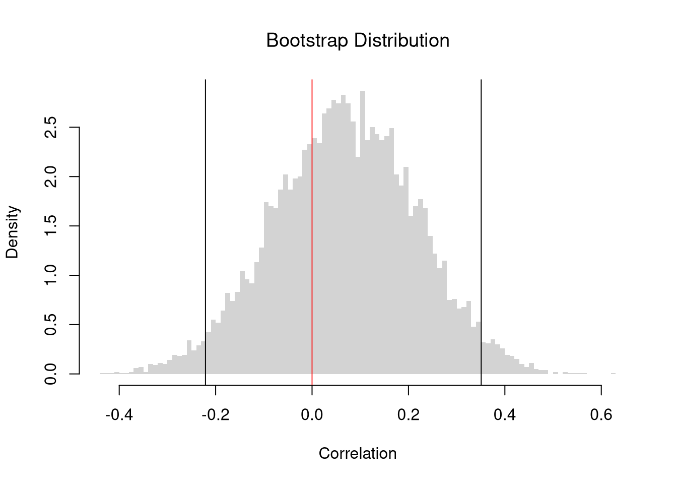
# Bootstrap Distribution of Correlation
n <- nrow(xy_hat)
bootstrap_cor <- rep(NA, 9999)
for(b in seq(bootstrap_cor) ){
    xy_boot <- xy_hat[sample(n, replace=TRUE), ]
    xy_cor_b <- cor(xy_boot[, 'x_hat'], xy_boot[, 'y_hat'])
    bootstrap_cor[b] <- xy_cor_b
}
hist(bootstrap_cor, breaks=100,
    border=NA, freq=FALSE,
    xlab='Correlation',
    main=NA)
title('Bootstrap Distribution', font.main=1)

## Test whether correlation is statistically different from 0
boot_ci <- quantile(bootstrap_cor, probs=c(0.025, 0.975))
abline(v=boot_ci)
abline(v=0, col=rgb(1, 0, 0, .8))

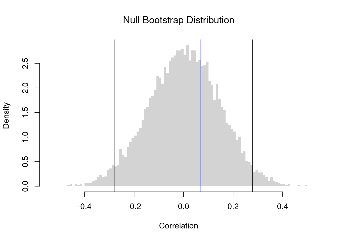
Importantly, we can also impose the null hypothesis of no association by reshuffling the data. If we resample without replacement, this is known as a permutation test.

Code
# xy_hat and xy_cor defined above
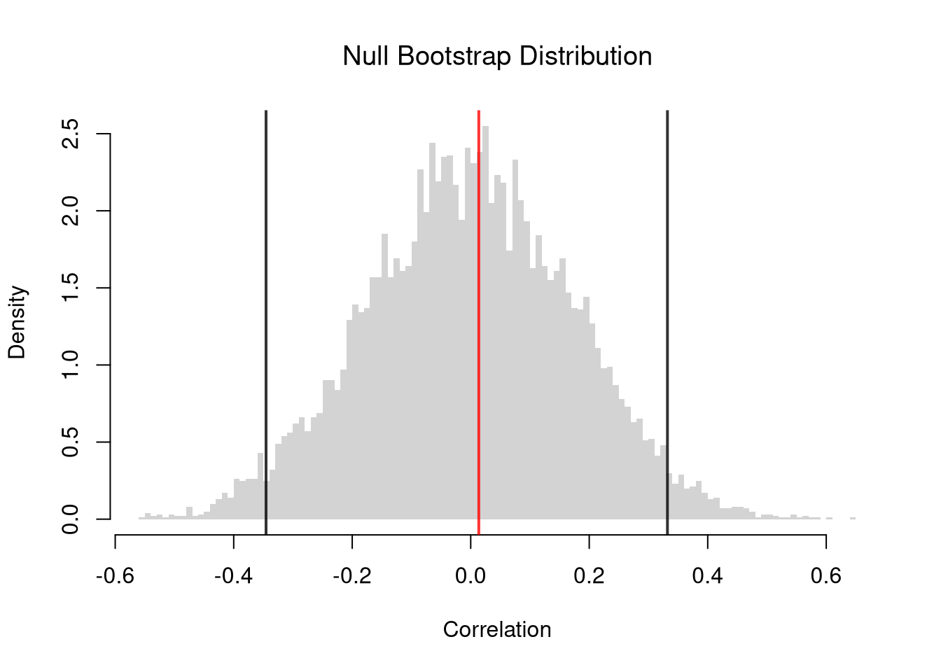
# Null Bootstrap Distribution of Correlation
n <- nrow(xy_hat)
null_bootstrap_cor <- rep(NA, 9999)
for(b in seq(null_bootstrap_cor) ){
    xy_boot <- xy_hat
    xy_boot[, 'x_hat'] <- xy_hat[sample(n, replace=TRUE), 'x_hat'] ## Reshuffle X
    xy_cor_b <- cor(xy_boot[, 'x_hat'], xy_boot[, 'y_hat'])
    null_bootstrap_cor[b] <- xy_cor_b
}
hist(null_bootstrap_cor, breaks=100,
    border=NA, freq=FALSE,
    xlab='Correlation',
    main=NA)
title('Null Bootstrap Distribution', font.main=1)

## Test whether correlation is statistically different from 0
boot_ci <- quantile(null_bootstrap_cor, probs=c(0.025, 0.975))
abline(v=boot_ci)
abline(v=xy_cor, col=rgb(0, 0, 1, .8))

All dependence resides in the pairing, and permuting one margin destroys the pairing completely.

To construct a permutation test, we need to use replace=FALSE. Rework the above code to make a Permutation Null Distribution and conduct a permutation test.

So the bootstrap evaluates sampling variability in the world that generated your data. A permutation test constructs the distribution of the statistic in a world where the null is true. Altogether, we have

Types of resampling
Distribution Sample Size per Iteration Number of Iterations Mechanism Typical Purpose
Jackknife \(n-1\) \(n\) \(X,Y\): Deterministically leave-one-out observation Variance estimate (after rescaling) and Normal CI estimate
Bootstrap \(n\) \(B\) \(X,Y\): Random resample with replacement Percentile CI estimate
Null Bootstrap \(n\) \(B\) \(X,Y\): Random resample with replacement and shifted Percentile CI under imposed null, \(p\)-values
Permutation \(n\) \(B\) \(X\): Random resample without replacement Percentile CI under imposed null of no association, \(p\)-values

Falk Codeviance

When the data contain outliers, the mean-based covariance can be misleading and a robust alternative is needed.

ImportantKey Definition

The Falk codeviance \(\tilde{C}_{XY}\) replaces the mean-based average in the covariance with the median of paired deviations from each variable’s median (where \(\tilde{m}_{X}\) and \(\tilde{m}_{Y}\) are the sample medians): \[\tilde{C}_{XY} = \text{Med}\left\{ (\hat{x}_{i} - \tilde{m}_{X})(\hat{y}_i - \tilde{m}_{Y}) \right\}.\]

The median correlation \(\tilde{R}_{XY}\) rescales the codeviance by the product of the two median absolute deviations: \[\tilde{R}_{XY} = \frac{ \tilde{C}_{XY} }{ \hat{\text{MAD}}_{X} \hat{\text{MAD}}_{Y}}.\]

The Falk codeviance is useful for cardinal data with outliers or heavy tails (income, prices, response times), where one extreme observation can move \(\hat{c}_{XY}\) by a lot but \(\tilde{C}_{XY}\) by very little (the same robustness rationale as for the median, \(IQR\), and \(\text{MAD}\) from Part 1).1 Unlike the Pearson correlation, the median correlation \(\tilde{R}_{XY}\) typically lies in \([-1,1]\) but not always.

Code
codev <- function(xy) {
  # Compute medians for each column
  med_hat <- apply(xy, 2, median)
  # Subtract the medians from each column
  xm <- sweep(xy, 2, med_hat, '-')
  # Return the median of the paired products
  CoDev <- median(xm[, 1] * xm[, 2])
  return(CoDev)
}
med_cor <- function(xy) {
  # Compute the medians of absolute deviation
  med_hat <- apply(xy, 2, median)
  xm <- sweep(xy, 2, med_hat, '-')
  MadProd <- prod( apply(abs(xm), 2, median) )
  # Return the robust correlation measure
  return( codev(xy) / MadProd)
}
xy_codev <- codev(xy_hat)
xy_codev
## [1] 0.25
xy_med_cor <- med_cor(xy_hat)
xy_med_cor
## [1] 0.005707763

Compute the Codeviance for the dataset \(\{(1,2),(2,1),(3,4),(4,3),(5,6)\}\).

The medians are \(\tilde{m}_{X}=3\) and \(\tilde{m}_{Y}=3\), giving signed deviations and products

\[\begin{array}{c|rrrrr} \hat{x}_{i}-\tilde{m}_{X} & -2 & -1 & 0 & 1 & 2 \\ \hat{y}_{i}-\tilde{m}_{Y} & -1 & -2 & 1 & 0 & 3 \\ (\hat{x}_{i}-\tilde{m}_{X})(\hat{y}_{i}-\tilde{m}_{Y}) & 2 & 2 & 0 & 0 & 6 \end{array}\]

The Codeviance is the median of those products: \(\tilde{C}_{XY}=\text{Med}\{0,0,2,2,6\}=2\). The median absolute deviations are \(\hat{\text{MAD}}_{X}=\text{Med}\{0,1,1,2,2\}=1\) and \(\hat{\text{MAD}}_{Y}=\text{Med}\{0,1,1,2,3\}=1\), so the median correlation is \(\tilde{R}_{XY}=2/(1\cdot1)=2\). Here \(\tilde{R}_{XY}\) exceeds \(1\): unlike Pearson’s correlation, the median correlation is not confined to \([-1,1]\).

Code
xy0_hat <- cbind(x_hat=c(1,2,3,4,5), y_hat=c(2,1,4,3,6))
codev(xy0_hat)
## [1] 2
med_cor(xy0_hat)
## [1] 2

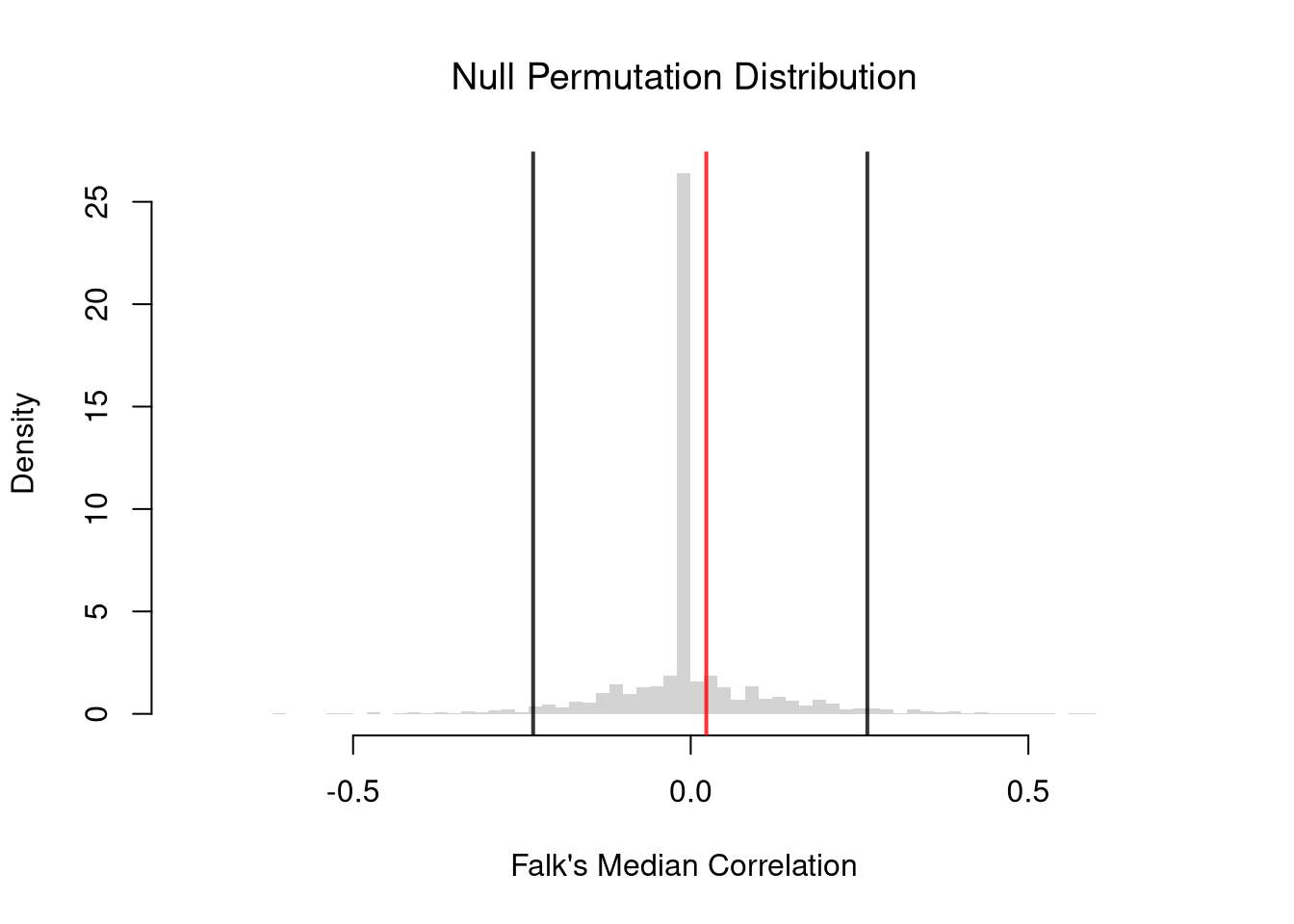
You construct sampling distributions and conduct hypothesis tests for Falk’s codeviance and the median correlation in the same way you do for Pearson’s Correlation statistic.

Code
# xy_hat and xy_med_cor defined above
# Null Permutation Distribution of the Median Correlation
n <- nrow(xy_hat)
null_permutation_med_cor <- rep(NA, 9999)
for(b in seq(null_permutation_med_cor) ){
    xy_perm <- xy_hat
    xy_perm[, 'x_hat'] <- xy_hat[sample(n, replace=FALSE), 'x_hat'] ## Reshuffle X
    xy_med_cor_b <- med_cor(xy_perm)
    null_permutation_med_cor[b] <- xy_med_cor_b
}
hist(null_permutation_med_cor, breaks=100,
    border=NA, freq=FALSE,
    xlab='Median Correlation',
    main=NA)
title('Null Permutation Distribution', font.main=1)

## Test whether the median correlation is statistically different from 0
abline(v=quantile(null_permutation_med_cor, probs=c(0.025, 0.975)))
abline(v=xy_med_cor, col=rgb(0, 0, 1, .8))

14.2 Factor Data

Two Ordered Factors

When the data are ordered (rankings or ordered categories), we can summarize association by counting which pairs of observations agree in direction.

ImportantKey Definition

Kendall’s rank correlation \(\hat{KT}\) is the share of variable-pairs that agree in direction (concordant) minus the share that disagree (discordant): \[\hat{KT} = \frac{2}{n(n-1)} \sum_{i} \sum_{j > i} \text{sgn} \Bigl( (\hat{x}_{i} - \hat{x}_{j})(\hat{y}_i - \hat{y}_j) \Bigr),\] where the sign function is \[\text{sgn}(z) = \begin{cases} +1 & \text{if } z > 0\\ 0 & \text{if } z = 0 \\ -1 & \text{if } z < 0 \end{cases}.\]

Kendall’s \(\hat{KT}\) is useful for any monotone relationship: the values do not have to fall on a straight line, only have consistent ordering. Because it only uses signs, it works for any ordinal data (rankings, ordered categories) where arithmetic averages are not meaningful. The bounds \([-1, 1]\) make it directly comparable to the Pearson correlation: a value closer to \(+1\) suggests positive association in rankings, \(-1\) negative, and \(0\) no association in the ordering. For example, consider years of schooling and wage brackets for the \(3294\) workers in Wages1. Both are ordered categories: \(12\) years is more than \(10\), and the top bracket pays more than the bottom one.

Code
# Load the Data
data(Wages1, package='Ecdat')
# Group hourly wages into four ordered brackets
wage_bracket <- cut(Wages1[, 'wage'], breaks=c(0, 4, 6, 8, Inf), ordered_result=TRUE)
xy_ord_hat <- data.frame(x_hat=Wages1[, 'school'], y_hat=wage_bracket) # x_hat=years of schooling, y_hat=wage bracket
table(xy_ord_hat)
##      y_hat
## x_hat (0,4] (4,6] (6,8] (8,Inf]
##    3      0     1     0       0
##    4      1     0     0       1
##    5      2     2     1       0
##    6      4     7     3       0
##    7     11     9     3       1
##    8     51    22     9       4
##    9     90    52    13       6
##    10   169   119    78      33
##    11   214   218   129     100
##    12   365   375   251     197
##    13    63    93    93      90
##    14    50    55    59     100
##    15    13    23    40      58
##    16     0     6     2       8

# Kendall's rank correlation uses only the order of the categories
KT <- cor(xy_ord_hat[, 'x_hat'], as.integer(xy_ord_hat[, 'y_hat']), method='kendall')
round(KT, 3)
## [1] 0.236

The value is positive, which suggests that workers with more schooling tend to be in higher wage brackets.

Kendall’s \(\hat{KT}\) also applies to cardinal data, because it only uses the ordering of the values. Converting each variable to ranks first does not change the statistic.

Code
# xy_hat defined above
# Convert each variable to ranks
xy_rank_hat <- xy_hat
xy_rank_hat[, 'x_hat'] <- rank(xy_hat[, 'x_hat'])
xy_rank_hat[, 'y_hat'] <- rank(xy_hat[, 'y_hat'])
# plot(xy_rank_hat, pch=16, col=grey(0, .25))
KT_rank <- cor(xy_rank_hat[, 'x_hat'], xy_rank_hat[, 'y_hat'], method = 'kendall')
round(KT_rank, 3)
## [1] 0.074
# Same value using the raw data
round(cor(xy_hat[, 'x_hat'], xy_hat[, 'y_hat'], method='kendall'), 3)
## [1] 0.074

Compute Kendall’s \(\hat{KT}\) for the dataset \(\{(1,1),(2,3),(3,2),(4,4)\}\).

With \(n=4\) there are \(n(n-1)/2=6\) pairs. For each pair we take the sign of \((\hat{x}_{i}-\hat{x}_{j})(\hat{y}_{i}-\hat{y}_{j})\): a pair is concordant (\(+1\)) if both variables move the same way, discordant (\(-1\)) if they move oppositely.

Pair \(X\) moves \(Y\) moves sign
(1,1),(2,3) up up \(+1\)
(1,1),(3,2) up up \(+1\)
(1,1),(4,4) up up \(+1\)
(2,3),(3,2) up down \(-1\)
(2,3),(4,4) up up \(+1\)
(3,2),(4,4) up up \(+1\)

There are \(5\) concordant and \(1\) discordant pair, so \[ \hat{KT} = \frac{2}{n(n-1)}\sum_{i}\sum_{j>i}\text{sgn}(\cdots) = \frac{2}{4\cdot3}(5-1) = \frac{8}{12} = \frac{2}{3} \approx 0.67. \]

Code
cor(c(1,2,3,4), c(1,3,2,4), method='kendall')
## [1] 0.6666667

You construct sampling distributions and conduct hypothesis tests for Kendall’s rank correlation statistic in the same way you do as for Pearson’s Correlation statistic and Falk’s Codeviance statistic.

Test whether Kendall’s correlation statistic is statistically different from \(0\). Expand on the example below to use bootstrapping.

Code
# xy_ord_hat defined above
KT <- cor(xy_ord_hat[, 'x_hat'], as.integer(xy_ord_hat[, 'y_hat']), method='kendall')

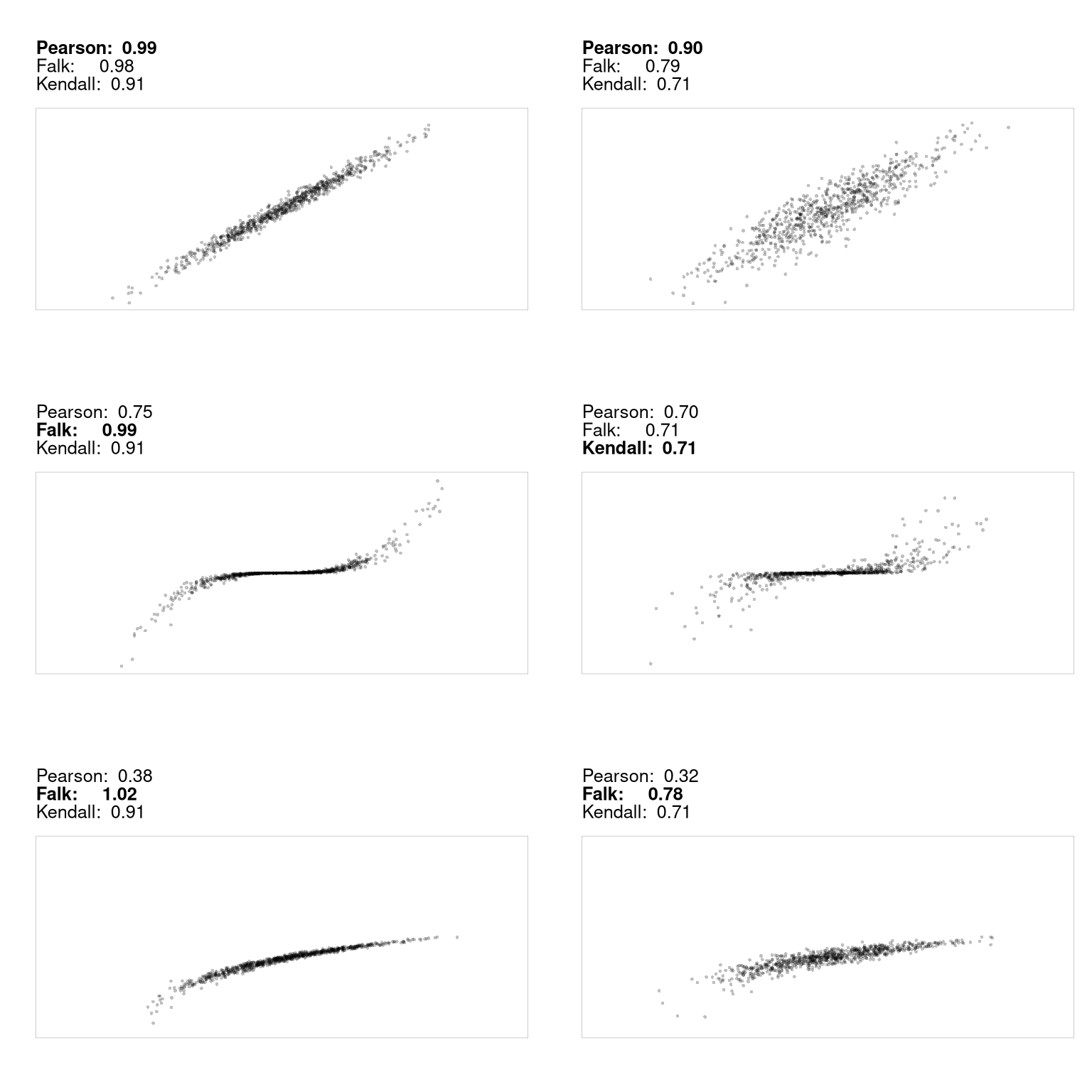
Kendall’s rank correlation coefficient can also be used for non-linear relationships, where Pearson’s correlation coefficient often falls short. It almost always helps to visualize your data first before summarizing it with a statistic.

Two Unordered Factors

When neither variable has a meaningful order, we organize the data as a contingency table and summarize the strength of association with a single bounded score.

ImportantKey Definition

Cramer’s V \(\hat{CV}\) rescales the chi-squared statistic \(\hat{\chi}^{2}\) into a \([0, 1]\) score for the strength of association between two categorical variables in a \(K\times J\) contingency table: \[\hat{\chi}^2 = \sum_{k=1}^{K} \sum_{j=1}^{J} \frac{(\hat{o}_{kj} - \hat{e}_{kj})^2}{\hat{e}_{kj}}, \qquad \hat{CV} = \sqrt{\frac{\hat{\chi}^2 / n}{\min(J - 1, \, K - 1)}},\] where \(\hat{o}_{kj}\) is the observed frequency in cell \((k, j)\), \(\hat{e}_{kj} = \hat{RF}_{k} \cdot \hat{CF}_{j} / n\) is the expected frequency under independence, and \(\hat{RF}_{k}=\sum_{j} \hat{o}_{kj}\), \(\hat{CF}_{j}=\sum_{k} \hat{o}_{kj}\) are the row and column totals.

Cramer’s V is useful for two unordered categorical variables (occupation, region, brand), because it treats every reordering of rows or columns the same and makes no use of any ordering. The chi-squared piece measures how far observed counts are from what we would expect if \(\hat{x}\) and \(\hat{y}\) were independent, and dividing by \(n \cdot \min(J - 1, K - 1)\) rescales it into a bounded score so different tables are comparable: \(0\) suggests no association, and a value closer to \(1\) suggests a strong association.

For example, consider the census region of each US state and its murder arrest rate grouped into three bands. Regions have no natural order, so we treat both variables as unordered categories. The state.region vector lists states in the same alphabetical order as the rows of USArrests.

Code
# Pair each state's region with its murder band (low, middle, high)
murder_band <- cut(USArrests[, 'Murder'], 3, labels=c('low', 'middle', 'high'))
xy_cat_hat <- data.frame(x_hat=state.region, y_hat=murder_band) # x_hat=census region, y_hat=murder band
table(xy_cat_hat)
##                y_hat
## x_hat           low middle high
##   Northeast       7      2    0
##   South           2      5    9
##   North Central   7      4    1
##   West            6      6    1

CV <- function(xy){
    # Create a contingency table from the categorical variables
    tbl <- table(xy)
    # Compute the chi-square statistic (without Yates' continuity correction)
    chi2 <- chisq.test(tbl, correct=FALSE)[['statistic']]
    # Total sample size
    n <- sum(tbl)
    # Compute the minimum degrees of freedom (min(rows-1, columns-1))
    df_min <- min(nrow(tbl) - 1, ncol(tbl) - 1)
    # Calculate Cramer's V
    V <- sqrt((chi2 / n) / df_min)
    return(V)
}
CV(xy_cat_hat)
## X-squared 
## 0.4497207

# DescTools::CramerV( table(xy_cat_hat) )

You can also apply Cramer’s V to cardinal data after cutting each variable into bins. This throws away the ordering of the bins, so Kendall’s \(\hat{KT}\) or Pearson’s \(\hat{r}_{XY}\) usually make better use of the data.

Code
# xy_hat and CV defined above
# Cut each variable into bins: UrbanPop into 4, Murder into 3
xy_bin_hat <- xy_hat
xy_bin_hat[, 'x_hat'] <- cut(xy_hat[, 'x_hat'], 4)
xy_bin_hat[, 'y_hat'] <- cut(xy_hat[, 'y_hat'], 3)
table(xy_bin_hat)
##              y_hat
## x_hat         (0.783,6.33] (6.33,11.9] (11.9,17.4]
##   (31.9,46.8]            4           0           2
##   (46.8,61.5]            5           4           4
##   (61.5,76.2]            8           7           2
##   (76.2,91.1]            5           6           3
CV(xy_bin_hat)
## X-squared 
## 0.2307071

Compute Cramer’s V for this \(2\times2\) table of \(100\) workers, cross-classifying a college degree against employment.

\[\begin{array}{c|cc|c} & \text{employed} & \text{unemployed} & \text{Row total}\\ \hline \text{degree} & 30 & 10 & 40\\ \text{no degree} & 20 & 40 & 60\\ \hline \text{Column total} & 50 & 50 & 100 \end{array}\]

If degree and employment were independent, the expected count in each cell is \(\hat{e}_{kj}=\hat{RF}_{k}\hat{CF}_{j}/n\). For the top-left cell, \(\hat{e}_{11}=40\cdot50/100=20\); all four expected counts are \((20,20,30,30)\). \[\begin{aligned} \hat{\chi}^2 &= \frac{(30-20)^2}{20}+\frac{(10-20)^2}{20}+\frac{(20-30)^2}{30}+\frac{(40-30)^2}{30} = 5+5+3.33+3.33 = 16.67. \end{aligned}\] With \(K=2\) rows and \(J=2\) columns, \(\min(J-1,K-1)=1\), so \[ \hat{CV} = \sqrt{\frac{\hat{\chi}^2/n}{\min(J-1,K-1)}} = \sqrt{\frac{16.67/100}{1}} \approx 0.41. \]

Code
# Observed 2x2 table
O <- rbind(degree    = c(employed=30, unemployed=10),
           no_degree = c(20, 40))
n0 <- sum(O)

# Expected counts under independence
E <- outer(rowSums(O), colSums(O)) / n0

# Chi-square statistic and Cramer's V
chi2 <- sum((O - E)^2 / E)
df_min <- min(nrow(O)-1, ncol(O)-1)
c(chi2=chi2, CramerV=sqrt((chi2/n0)/df_min))
##       chi2    CramerV 
## 16.6666667  0.4082483

You construct sampling distributions and conduct hypothesis tests for Cramer’s V statistic in the same way you do as the other statistics.

14.3 Exercises

  1. Comment the script you wrote for this chapter, then restart R and check that it runs from a clean session, then check the script with AI as explained in Working with AI. Write three sentences from memory on the main statistical idea of this chapter, and ask the assistant what is wrong, vague, or missing. Finish with your own questions about whatever you found hardest.

  2. For the dataset \(\{(1, 5),\ (2, 3),\ (3, 4),\ (4, 2),\ (5, 1)\}\), compute the Pearson correlation \(\hat{r}_{XY}\) by hand. Show all five steps: means, deviances, covariance \(\hat{c}_{XY}\), standard deviations \(\hat{s}_{X}\) and \(\hat{s}_{Y}\), and the final correlation.

  3. Using the USArrests dataset, compute both the Pearson correlation and Kendall’s rank correlation between Murder and Assault. Then write a bootstrap with \(B = 9999\) iterations to construct a \(95\%\) confidence interval for the Pearson correlation. Does the interval contain zero?

Further Reading

Recall

This chapter summarized two-variable association with a small toolbox matched to data type: Pearson correlation \(\hat{r}_{XY}\) for cardinal data (worked out by hand on \(\{(0, 0.1), (1, 0.3), (2, 0.2)\}\), yielding \(\hat{r}_{XY}=1/2\)), Falk codeviance \(\tilde{C}_{XY}\) as the robust cousin for outlier-prone data, Kendall’s \(\hat{KT}\) for ordered factors (walked through the six pairs of \(\{(1, 1), (2, 3), (3, 2), (4, 4)\}\) to get \(\hat{KT}=2/3\)), and Cramer’s V \(\hat{CV}\) for unordered factors (the \(2\times 2\) degree-vs-employment table giving \(\hat{CV}\approx 0.41\)). These statistics describe association rather than causation.


  1. See Medians and Absolute Deviations. See also the Theil-Sen Estimator, which may be seen as a precursor.↩︎