17  Inference


Often, we are interested in gradients: how \(Y\) changes with \(X\). The linear model from Simple Regression depicts this as a single constant, \(\hat{b}_{1}\), but the local-regression models from Local Regression do not. A great first step to assess gradients is to plot the predicted values over the explanatory values. A great second step is to compute gradients and summarize them. In any case, we compute confidence intervals to account for variability across samples.

17.1 Applied Methods

LOESS

When \(\hat{x}_{i}\) is unevenly distributed across its range, a fixed bandwidth \(h\) leaves some local fits with many neighbors and others with very few.

ImportantKey Definition

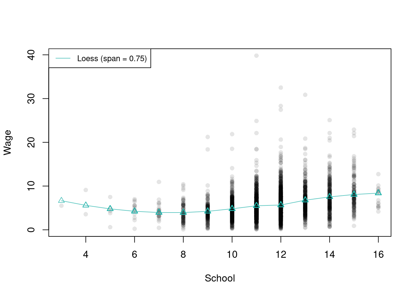
LOESS (locally estimated scatterplot smoothing) fits a local linear (or quadratic) regression at each design point using an adaptive bandwidth: instead of fixing \(h\), it includes a fixed share of the data at each \(x\), set by the parameter span.

LOESS is useful for smoothing data with uneven \(X\): because the share of points in each neighborhood is fixed, the local fit has roughly the same effective sample size everywhere, even where the data are sparse. The span parameter plays the role \(h\) does for fixed-bandwidth methods, so smaller spans mean narrower neighborhoods, more flexibility, and noisier curves, while larger spans pool more data and smooth more aggressively.

Code
## Data
library(Ecdat)
xy2_hat <- Wages1[order(Wages1[, 'school']), c('school', 'wage')]
colnames(xy2_hat) <- c('x_hat', 'y_hat') # x_hat=years of schooling, y_hat=hourly wage

# Fit loess with the default span
reg_lo <- loess(y_hat ~ x_hat, data=xy2_hat)

plot(y_hat ~ x_hat, pch=16, col=grey(0, .1), data=xy2_hat,
    main=NA, xlab='School', ylab='Wage')
lo_col <- adjustcolor('#20B2AA', alpha.f=.75)  # teal green
lines(xy2_hat[, 'x_hat'], predict(reg_lo),
    col=lo_col, type='o', pch=2)

legend('topleft',
    legend=sprintf('Loess (span = %.2f)', reg_lo$pars$span),
    lty=1, col=lo_col, cex=.8)

Confidence Bands

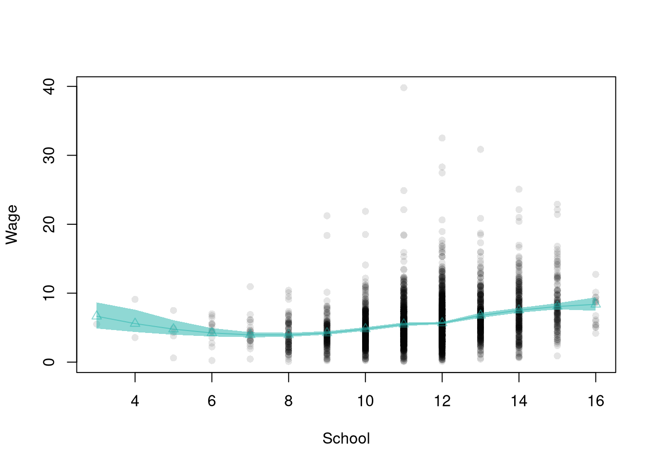
A single fitted curve does not show how much that curve would change in another sample, so we draw a region around it.

ImportantKey Definition

A confidence band is a confidence interval drawn at every design point: a region around the fitted curve that captures sample-to-sample variability. A bootstrap confidence band collects the predictions from many resamples and reads off pointwise quantiles at each \(x\).

Confidence bands are useful for showing where a fitted curve is well-supported by the data and where another sample could move it. The width is typically wider at the edges of \(X\) (few neighbors) and narrower in the dense middle, which is itself a quick visual diagnostic. The same bootstrap that produces the band also produces standard errors for any single design point and for the gradient summaries below.

Code
# Same loess fit as above (default span)
pred_design <- data.frame(x_hat=unique(xy2_hat[, 'x_hat']))
y_fit <- predict(reg_lo, newdata=pred_design)

plot(y_hat ~ x_hat, pch=16, col=grey(0, .1), data=xy2_hat,
    main=NA, xlab='School', ylab='Wage')
lo_col <- adjustcolor('#20B2AA', alpha.f=.5)  # same teal green
lines(pred_design[, 'x_hat'], y_fit,
    col=lo_col, type='o', pch=2)

# Boot CI with the same default-span loess
boot_lo <- matrix(NA, nrow=nrow(pred_design), ncol=399)
for (b in 1:399) {
    xy2_boot <- xy2_hat[sample(nrow(xy2_hat), replace=TRUE), ]
    reg_b <- loess(y_hat ~ x_hat, data=xy2_boot)
    boot_lo[, b] <- predict(reg_b, newdata=pred_design)
}
boot_cb <- apply(boot_lo, 1, quantile,
    probs=c(.025, .975), na.rm=TRUE)

# Plot CI
polygon(
    c(pred_design[[1]], rev(pred_design[[1]])),
    c(boot_cb[1, ], rev(boot_cb[2, ])),
    col=lo_col,
    border=NA)

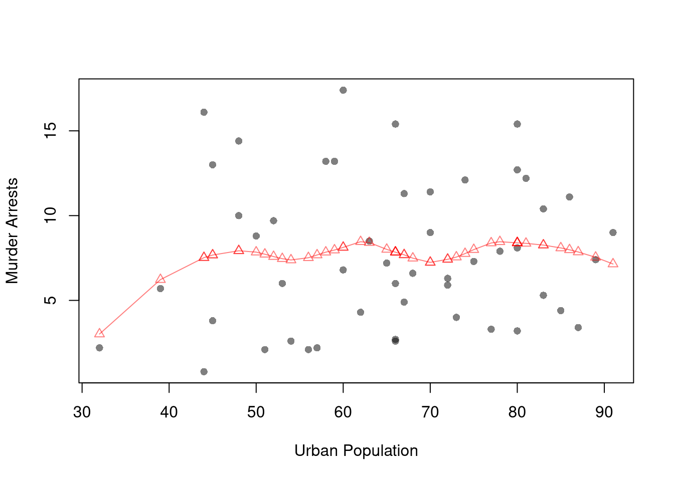
Construct a bootstrap confidence band for the following loess regression

Code
# Adaptive-width subsamples with non-uniform weights
xy_hat <- USArrests[, c('UrbanPop', 'Murder')]
colnames(xy_hat) <- c('x_hat', 'y_hat') # x_hat=urban population share, y_hat=murder arrests per 100K
xy_ord_hat <- xy_hat[order(xy_hat[, 'x_hat']), ]

plot(y_hat ~ x_hat, pch=16, col=grey(0, .5), data=xy_ord_hat,
    main=NA, xlab='Urban Population', ylab='Murder Arrests')
reg_lo_usa <- loess(y_hat ~ x_hat, data=xy_ord_hat, span=.6)

red_col <- rgb(1, 0, 0, .5)
lines(xy_ord_hat[, 'x_hat'], predict(reg_lo_usa),
    col=red_col, type='o', pch=2)

Bias-Variance Tradeoff

A better fit on the data you have is not automatically better, because a model can hit every point in the sample and still predict new observations poorly.

ImportantKey Definition

The bias-variance tradeoff describes two sources of model error: bias (systematic miss from over-smoothing) and variance (sample-to-sample wobble from under-smoothing).

The bias-variance tradeoff is useful for thinking about why a tuning parameter matters and how to set it. For local regressions, the bandwidth \(h\) (equivalently, the LOESS span) is the lever that governs the tradeoff: large \(h\) trades variance down for bias up, small \(h\) does the opposite. A loess fit narrow enough to interpolate every point has \(\hat{MSE}=0\) on the fit data but generalizes poorly because it has just copied the noise.

  • Wide window (large span, large \(h\)): each local fit uses many observations, so the fitted curve barely changes from sample to sample (low variance). But a nearly flat fit over a wide region cannot follow a relationship that bends, so it is systematically off (high bias).
  • Narrow window (small span, small \(h\)): each local fit uses few observations, so the fitted curve chases noise and swings from sample to sample (high variance). But a narrow window can track curvature closely (low bias).
Code
# Two-span loess with bootstrap confidence bands on one scatterplot
pred_design <- data.frame(x_hat=sort(unique(xy2_hat[, 'x_hat'])))
spans <- c(4.0, 0.4)
n_boot <- 399
span_col <- hcl.colors(3, alpha=.9)[c(1, 3)]

plot(y_hat ~ x_hat, data=xy2_hat, pch=16, col=grey(0, .1),
    main=NA, xlab='School', ylab='Wage')

for (s in seq_along(spans)) {
    sp <- spans[s]
    reg_s <- loess(y_hat ~ x_hat, data=xy2_hat, span=sp)
    boot_preds <- matrix(NA, nrow=nrow(pred_design), ncol=n_boot)
    for (b in 1:n_boot) {
        xy2_boot <- xy2_hat[sample(nrow(xy2_hat), replace=TRUE), ]
        reg_s_b <- loess(y_hat ~ x_hat, data=xy2_boot, span=sp)
        boot_preds[, b] <- predict(reg_s_b, newdata=pred_design)
    }
    boot_cb <- apply(boot_preds, 1, quantile,
        probs=c(.025, .975), na.rm=TRUE)

    polygon(c(pred_design[, 'x_hat'], rev(pred_design[, 'x_hat'])),
        c(boot_cb[1, ], rev(boot_cb[2, ])),
        col=adjustcolor(span_col[s], alpha.f=0.3), border=NA)
    lines(pred_design[, 'x_hat'], predict(reg_s, newdata=pred_design),
        col=span_col[s], lwd=2)
}

legend('topleft', title='LOESS span',
    legend=paste0(spans),
    col=span_col, lty=1, lwd=2, cex=.8)

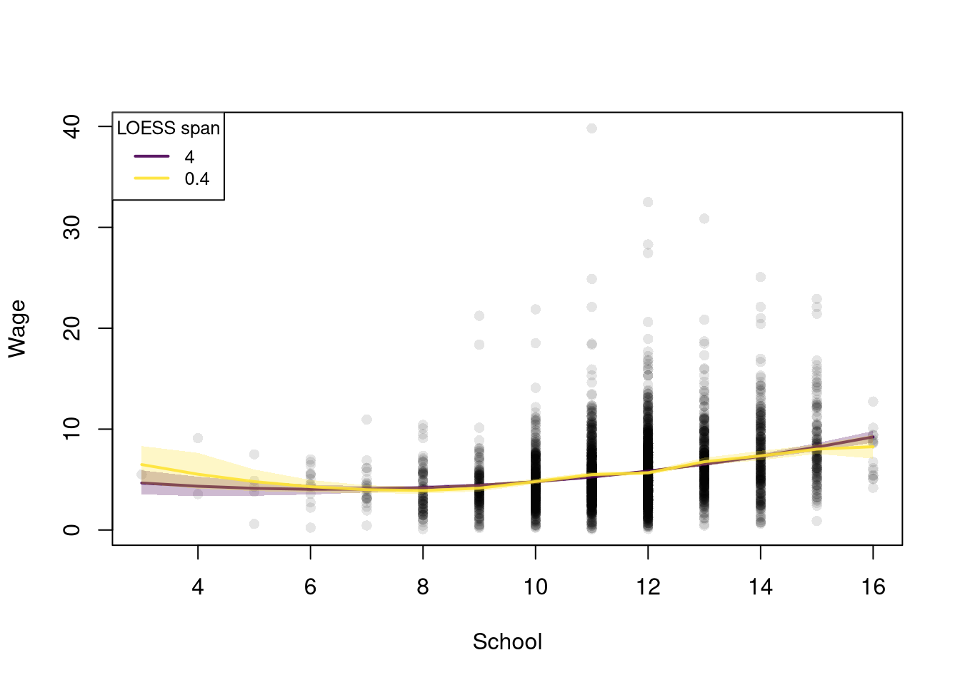
With span \(4.0\) the fitted curve is very smooth and stable, and the bootstrap band sits tightly around it. With span \(0.4\) the curve tracks more local variation, and the bootstrap band fans wider, directly displaying the variance penalty for chasing local detail. (Schooling x_hat is integer-valued with only \(14\) distinct values, so spans below about \(0.4\) collapse to single-point neighborhoods and loess() cannot fit.)

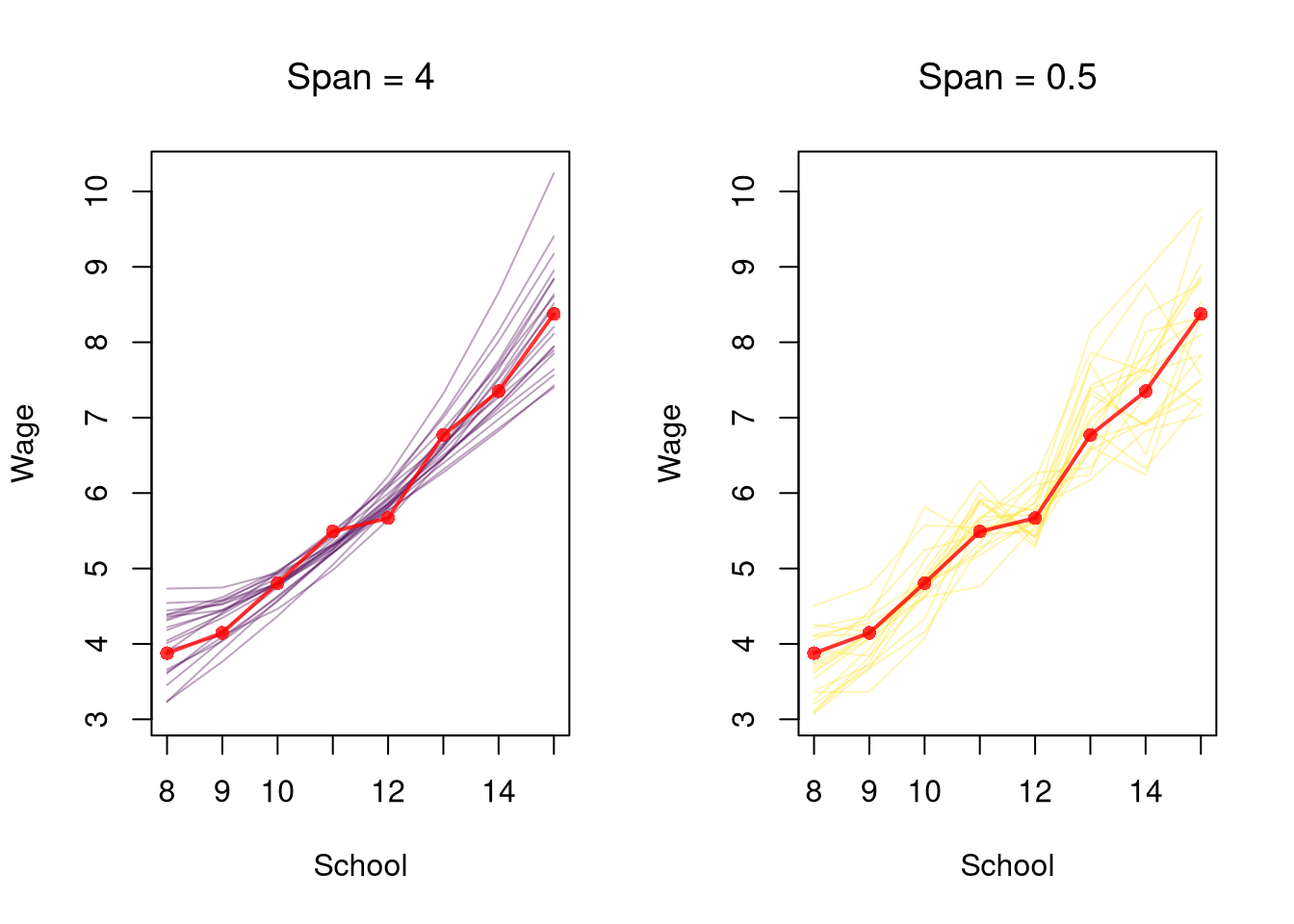
The bootstrap bands show variance, but not bias, because we never see the true curve in one sample. As in Sampling, pretend the \(3294\) workers in Wages1 are the whole population, so the true curve is known. The population curve is the mean wage at each schooling level over all \(3294\) workers. We then draw many samples of \(n=300\) workers, fit a wide span (\(4.0\)) and a narrow span (\(0.5\)) to each, and see how the fitted curves compare to the population curve. At \(n=300\), span \(0.4\) sometimes fails, so we use \(0.5\) for the narrow window.

Code
# Pretend these 3294 workers are the whole population
data(Wages1, package='Ecdat')
population_xy <- Wages1[, c('school', 'wage')]
colnames(population_xy) <- c('x', 'y') # x=years of schooling, y=hourly wage
population_slope <- coef(lm(y ~ x, data=population_xy))[2]

# Population curve: mean wage at each schooling level
population_curve <- tapply(population_xy[, 'y'], population_xy[, 'x'], mean)

# Evaluate at schooling levels with many workers (8 to 15 years)
# Rare levels are often missing from a sample, and loess does not extrapolate
x_levels <- 8:15
population_levels <- population_curve[as.character(x_levels)]

# Repeated samples, each fit with a wide and a narrow span
spans_sim <- c(4.0, 0.5)
n <- 300
n_rep <- 200
curves_sim <- array(NA, dim=c(length(x_levels), n_rep, length(spans_sim)))
for (r in 1:n_rep) {
    s_id <- sample(nrow(population_xy), n, replace=FALSE)
    xy_sim <- population_xy[s_id, ]
    colnames(xy_sim) <- c('x_hat', 'y_hat')
    for (s in seq_along(spans_sim)) {
        # Return NA if loess fails on this sample
        curves_sim[, r, s] <- tryCatch(
            suppressWarnings(predict(
                loess(y_hat ~ x_hat, data=xy_sim, span=spans_sim[s]),
                newdata=data.frame(x_hat=x_levels))),
            error=function(e) rep(NA, length(x_levels)))
    }
}

# Plot a few sample curves for each span, plus the population curve
par(mfrow=c(1, 2))
for (s in seq_along(spans_sim)) {
    matplot(x_levels, curves_sim[, 1:20, s], type='l', lty=1,
        col=adjustcolor(span_col[s], alpha.f=.4),
        ylim=range(curves_sim[, 1:20, ], population_levels, na.rm=TRUE),
        xlab='School', ylab='Wage', main=NA)
    lines(x_levels, population_levels, col=rgb(1, 0, 0, .8), lwd=2, type='o', pch=16)
    title(paste0('Span = ', spans_sim[s]), font.main=1)
}

Each thin line is the fit from one sample, and the red line is the population curve. The wide-span curves stay close to one another, but they are too straight to follow the bend in the population curve. The narrow-span curves follow the bend better on average, but they spread out much more from sample to sample.

We can summarize this with two numbers per span. At each schooling level, the squared bias is the squared gap between the average fitted value and the population curve, and the variance is the spread of the fitted values across samples. We then average each over the schooling levels.

Code
# Average squared bias and variance across schooling levels
bias_var <- sapply(seq_along(spans_sim), function(s) {
    curves_s <- curves_sim[, , s]
    bias2_s <- (rowMeans(curves_s, na.rm=TRUE) - population_levels)^2
    var_s <- apply(curves_s, 1, var, na.rm=TRUE)
    c(Bias2=mean(bias2_s), Variance=mean(var_s), MSE=mean(bias2_s + var_s))
})
colnames(bias_var) <- paste0('Span ', spans_sim)
round(bias_var, 3)
##          Span 4 Span 0.5
## Bias2     0.034    0.009
## Variance  0.128    0.301
## MSE       0.162    0.310

The wide span typically has the larger squared bias and the smaller variance, while the narrow span has the opposite. Here the variance term is the larger of the two, so the wide span often has the lower total error at \(n=300\). With a larger sample, the variance of both fits falls, and the narrow span becomes more attractive. Choosing the span (the bandwidth \(h\)) means trading bias against variance.

Note that when the local fits are linear (degree=1), the simple linear regression is nested as a special case with \(span \to \infty\), because every observation then gets nearly the same weight. By default, loess() fits local quadratics (degree=2), so a very wide default fit approaches a global quadratic instead of a straight line.

Model Fit

Each local model produces fitted values \(\hat{y}_{i}^{\mathrm{fit}}\) and residuals \(\hat{e}_{i} = \hat{y}_{i} - \hat{y}_{i}^{\mathrm{fit}}\). To compare models, we often summarize the residuals with a single number.

The mean squared error averages the squared residuals, \[\begin{aligned} \hat{MSE} &= \frac{1}{n}\sum_{i=1}^{n} \hat{e}_{i}^2 = \frac{1}{n}\sum_{i=1}^{n} \left(\hat{y}_{i} - \hat{y}_{i}^{\mathrm{fit}}\right)^2. \end{aligned}\] Squaring penalizes large misses heavily, and the units are the square of \(\hat{y}_{i}\) (squared dollars for wages).

The mean absolute percentage error instead averages each residual relative to its observed value, \[\begin{aligned} \hat{MAPE} &= \frac{100}{n}\sum_{i=1}^{n} \left| \frac{\hat{e}_{i}}{\hat{y}_{i}} \right|. \end{aligned}\] MAPE is unit-free, which makes it easy to communicate, but it is undefined when \(\hat{y}_{i}=0\) and over-weights observations with small \(\hat{y}_{i}\). MSE is easier to analyze theoretically (formally deriving the bias-variance tradeoff)

Suppose three workers have wages \(\hat{y}=(8, 10, 15)\) and a model predicts \(\hat{y}^{\mathrm{fit}}=(9, 9, 14)\). The residuals are \(\hat{e}=(-1, 1, 1)\), so \[\begin{aligned} \hat{MSE} &= \frac{(-1)^2 + 1^2 + 1^2}{3} = \frac{3}{3} = 1, \\ \hat{MAPE} &= \frac{100}{3}\left( \frac{1}{8} + \frac{1}{10} + \frac{1}{15} \right) \approx \frac{100}{3}(0.292) \approx 9.7. \end{aligned}\] The model misses by \(1\) squared-dollar on average, or about \(10\%\) of each wage.

Code
y0_hat <- c(8, 10, 15)
y0_fit <- c(9, 9, 14)
e0_hat <- y0_hat - y0_fit
mean(e0_hat^2)           # MSE
## [1] 1
100*mean(abs(e0_hat/y0_hat))  # MAPE
## [1] 9.722222

We can compute these for the linear, regressogram, and piecewise models on the wage~school data.

Code
# xy2_hat defined above

# Three models for wage on schooling
reg_lin <- lm(y_hat ~ x_hat, data=xy2_hat)        # globally linear
xy2_hat[, 'xcf'] <- cut(xy2_hat[, 'x_hat'], 3)
reg_rgram <- lm(y_hat ~ xcf, data=xy2_hat)         # regressogram, 3 bins
reg_pw    <- lm(y_hat ~ xcf*x_hat, data=xy2_hat)  # piecewise, 3 bins

# Mean squared error and mean absolute percentage error
fit_stats <- function(model){
    e_hat <- resid(model)
    y_hat <- xy2_hat[, 'y_hat']
    c(MSE=mean(e_hat^2), MAPE=100*mean(abs(e_hat/y_hat)))
}
round(rbind(
    Linear       = fit_stats(reg_lin),
    Regressogram = fit_stats(reg_rgram),
    Piecewise    = fit_stats(reg_pw)), 2)
##                MSE  MAPE
## Linear        9.83 73.27
## Regressogram 10.27 75.88
## Piecewise     9.73 72.82
17.2 Relationships

Gradients

Once the fitted curve can bend, “the slope” is no longer a single number; we want the slope locally at each \(x\).

ImportantKey Definition

A gradient \(\hat{b}_{1}(x)\) at the design point \(x\) is the rate of change of the fitted value \(\hat{y}^{\mathrm{fit}}(x)\) with respect to \(\hat{x}_{i}\) in a neighborhood of \(x\).

The gradient is useful as the local analog of the simple-regression slope: for a globally linear model it equals the single coefficient \(\hat{b}_{1}\) everywhere; for a local model it varies with \(x\) and traces out how the marginal relationship changes across the range of \(X\). Three common ways to summarize gradients are:

  1. For all methods, including regressograms, you can approximate gradients with small finite differences. For some small difference \(d\), we can manually compute \[\begin{aligned} \hat{b}_{1}(x) &= \frac{ \hat{y}^{\mathrm{fit}}(x+\frac{d}{2}) - \hat{y}^{\mathrm{fit}}(x-\frac{d}{2})}{d}, \end{aligned}\]

  2. When using split-sample regressions or local linear regressions, you can use the estimated slope coefficients \(\hat{b}_{1}(x)\) as a gradient estimate.1

  3. More sophisticated methods that are beyond the scope of this class.

Suppose a local model predicts wages near \(x=12\) years of schooling: \(\hat{y}^{\mathrm{fit}}(11.5)=9.2\) and \(\hat{y}^{\mathrm{fit}}(12.5)=10.4\) (dollars per hour). With step \(d=1\), the finite-difference gradient at \(x=12\) is \[ \hat{b}_{1}(12) = \frac{\hat{y}^{\mathrm{fit}}(12.5) - \hat{y}^{\mathrm{fit}}(11.5)}{d} = \frac{10.4 - 9.2}{1} = 1.2. \] Near \(12\) years of schooling, each extra year is associated with about \(\$1.20\) more per hour.

Code
d <- 1
y_fit_hi <- 10.4  # prediction at x + d/2
y_fit_lo <- 9.2   # prediction at x - d/2
(y_fit_hi - y_fit_lo) / d
## [1] 1.2

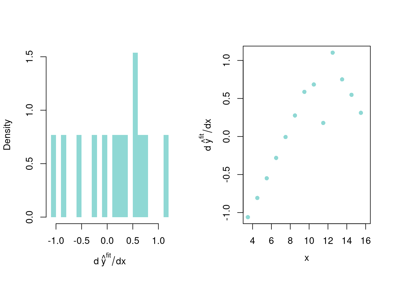
After computing gradients, you can summarize them in various plots: Histograms and Scatterplots. The confidence band only shows variability across samples, whereas these plots show variability within-sample. You can also plot all Gradients with their CI’s (Chaudhuri and Marron 1999; Henderson et al. 2012).

Code
## Gradients
y_fit <- predict(reg_lo)
grad_dx <- diff(xy2_hat[, 'x_hat'])
grad_dy <- diff(y_fit)
grad_lo <-grad_dy/grad_dx

## Visual Summary
par(mfrow=c(1, 2))
hist(grad_lo,  breaks=20,
    border=NA, freq=FALSE,
    col=lo_col,
    xlab=expression(d~hat(y)^plain(fit)/dx),
    main=NA) ## Distributional Summary
  
## Visual Summary 2
grad_x  <- xy2_hat[-nrow(xy2_hat), 'x_hat'] + grad_dx/2 # midpoint of consecutive x
plot(grad_x, grad_lo,
    xlab='x', ylab=expression(d~hat(y)^plain(fit)/dx),
    mgp=c(2.5, 1, 0),
    col=lo_col, pch=16, main=NA) ## Diminishing Returns?

A different kind of summary collapses the whole gradient curve into a single number for tabular reporting.

ImportantKey Definition

The gradient at the mean (sometimes called the marginal effect at the mean) evaluates the gradient at a single design point: \[\hat{b}_{1}(x=\hat{m}_{X}).\] The mean of the gradients (sometimes called the average effect or mean marginal effect) averages \(\hat{b}_{1}(x)\) across every observation in the dataset: \[\frac{1}{n}\sum_{i=1}^{n} \hat{b}_{1}(x=\hat{x}_{i}).\]

These two summaries are useful for different questions: the gradient at the mean answers “what is the slope at a typical \(X\)?”, while the mean of the gradients answers “what is the average slope across the sample?”. The two coincide for a globally linear model but can differ for any other, sometimes substantially when the relationship bends. You may also be interested in the median of the gradients, or in measures of effect heterogeneity like the interquartile range or standard deviation of the gradients. Such statistics can be presented in tabular form: “mean gradient (sd gradient)” or “mean gradient (estimated SE), sd gradient (estimated SE)”.

These two summaries usually differ. Suppose a local model has gradients \(\hat{b}_{1}(x)\) at schooling levels \(x=(8,10,12,14,16)\) equal to \((0.4, 0.8, 1.2, 0.9, 0.3)\), and the sample mean schooling is \(\hat{m}_{X}=12\).

  • The marginal effect at the mean is the single gradient at \(x=\hat{m}_{X}\): \(\hat{b}_{1}(12) = 1.2\).
  • The mean of the gradients averages over all five points: \(\frac{0.4+0.8+1.2+0.9+0.3}{5} = \frac{3.6}{5} = 0.72\).

They differ because the gradient is not constant: here the relationship is steepest near the mean and flatter at the extremes.

Code
grads <- c(0.4, 0.8, 1.2, 0.9, 0.3)
grads[3]      # marginal effect at the mean (x = 12)
## [1] 1.2
mean(grads)   # mean of the gradients
## [1] 0.72
Code
## Tabular Summary
tab_stats <- c(
    Mean=mean(grad_lo, na.rm=TRUE),
    SD=sd(grad_lo, na.rm=TRUE))

## Use bootstrap to approximate sampling dist
boot_stats <- matrix(NA, nrow=299, ncol=2)
colnames(boot_stats) <- c('Mean', 'SD')
for(b in 1:nrow(boot_stats)){
    xy2_boot <- xy2_hat[sample(1:nrow(xy2_hat), replace=TRUE), ]
    xy2_boot <- xy2_boot[order(xy2_boot[, 'x_hat']), ] # sort so diff() runs along x
    reg_lo_b <- loess(y_hat ~ x_hat, data=xy2_boot)
    y_fit_b <- predict(reg_lo_b)
    grad_lo_b <- diff(y_fit_b)/diff(xy2_boot[, 'x_hat'])
    m_grad_b_hat <- mean(grad_lo_b, na.rm=TRUE)
    s_grad_b_hat <- sd(grad_lo_b, na.rm=TRUE)
    boot_stats[b, 1] <- m_grad_b_hat
    boot_stats[b, 2] <- s_grad_b_hat
}
## SEs and CIs
boot_se <- apply(boot_stats, 2, sd)
boot_quants <- apply(boot_stats, 2, quantile, probs=c(0.025, 0.975))
boot_quants <- apply( round(boot_quants, 3), 2, paste0, collapse=', ')

## Printing
tab_regstyle <- data.frame(
  Estimate  = round(tab_stats, 3),
  SE = paste0('(', round(boot_se, 3), ')'),
  CI_95 = paste0('[', boot_quants, ']')
)
tab_regstyle
##      Estimate      SE          CI_95
## Mean    0.133 (0.091) [0.004, 0.352]
## SD      0.647 (0.105) [0.432, 0.835]
Summary of Local Gradients
Estimate Bootstrap.SE Bootstrap.95.CI
Mean 0.13 (0.091) [0.004, 0.352]
SD 0.65 (0.105) [0.432, 0.835]

Hypothesis Testing

We can test whether the mean gradient is statistically different from zero. We can compute the p-value directly from the bootstrap distribution. Under \(H_0\), the mean gradient equals zero, so we center the bootstrap distribution at zero and ask how often it produces values as extreme as the observed mean gradient.

Code
## P-value via null bootstrap ECDF
## Center bootstrap means at zero (impose H0)
boot_centered <- boot_stats[, 'Mean'] - mean(boot_stats[, 'Mean'])

## ECDF of centered bootstrap distribution
F_hat <- ecdf(boot_centered)

## Two-sided p-value: P(|centered mean| >= |observed mean|)
p_boot <- 1 - F_hat(abs(tab_stats['Mean'])) +
              F_hat(-abs(tab_stats['Mean']))

cat('Bootstrap p-value (ECDF):', format.pval(p_boot, digits=3), '\n')
## Bootstrap p-value (ECDF): 0.151

The small p-value indicates that the mean gradient is statistically distinguishable from zero: on average, wages increase with schooling.

We can also use a normal approximation. Under the null hypothesis \(H_0\): the mean gradient equals zero, we use the test statistic \[t = \frac{\text{mean gradient}}{\text{SE(mean gradient)}}\] and the p-value comes from the standard normal distribution.

Code
## P-value for mean gradient
## Standard Normal Approximation
t_stat <- tab_stats['Mean'] / boot_se['Mean']
p_val  <- 2 * pnorm(-abs(t_stat))

cat('Mean gradient:', round(tab_stats['Mean'], 3), '\n')
## Mean gradient: 0.133
cat('Bootstrap SE: ', round(boot_se['Mean'], 3), '\n')
## Bootstrap SE:  0.091
cat('t-statistic:  ', round(t_stat, 3), '\n')
## t-statistic:   1.466
cat('p-value:      ', format.pval(p_val, digits=3), '\n')
## p-value:       0.143

Compute the t-statistic and p-value using jackknife standard errors instead of the bootstrap.

Code
## Jackknife SE for mean gradient
n <- nrow(xy2_hat)
jack_means <- numeric(n)
for (i in 1:n) {
    xy2_i  <- xy2_hat[-i, ]
    reg_i  <- loess(y_hat ~ x_hat, data=xy2_i)
    y_fit_i <- predict(reg_i)
    grad_i <- diff(y_fit_i) / diff(xy2_i[, 'x_hat'])
    jack_means[i] <- mean(grad_i, na.rm=TRUE)
}

## Jackknife SE
jack_se <- sqrt((n - 1) / n * sum((jack_means - mean(jack_means))^2))

## t-statistic and p-value
t_jack <- tab_stats['Mean'] / jack_se
p_jack <- 2 * pnorm(-abs(t_jack))

cat('Jackknife SE: ', round(jack_se, 3), '\n')
## Jackknife SE:  0.12
cat('t-statistic:  ', round(t_jack, 3), '\n')
## t-statistic:   1.114
cat('p-value:      ', format.pval(p_jack, digits=3), '\n')
## p-value:       0.265

17.3 Exercises

  1. Comment the script you wrote for this chapter, then restart R and check that it runs from a clean session, then check the script with AI as explained in Working with AI. Write three sentences from memory on the main statistical idea of this chapter, and ask the assistant what is wrong, vague, or missing. Finish with your own questions about whatever you found hardest.

  2. A linear regression has low variance but can have high bias when the true relationship is nonlinear. A loess regression with a small span has low bias but high variance. Explain why increasing the sample size \(n\) helps reduce the standard error for both models, but only helps reduce bias for loess (with an appropriate bandwidth rule).

  3. Using the USArrests dataset, fit a loess regression of Murder on UrbanPop with span = 0.6. Compute the finite-difference gradients \(\hat{b}_{1}(x)\) and report their mean and standard deviation. Compare these to the OLS slope \(\hat{b}_{1}\) from a simple linear regression.

  4. Using the USArrests dataset and the loess fit from the previous question, write R code to construct a bootstrap confidence band with \(B = 399\) replicates. Plot the scatterplot, the loess curve, and the shaded 95% confidence band.

Further Reading

Recall

This chapter put inference around the local fits from the previous chapter on the Wages1 data: model-fit metrics (\(\hat{MSE}\) and \(\hat{MAPE}\)) and the bias-variance tradeoff, bootstrap confidence bands for a LOESS fit, gradient summaries (marginal effect at the mean vs mean of the gradients), and hypothesis tests. The small worked example with \(\hat{y}^{\mathrm{fit}}(11.5)=9.2\) and \(\hat{y}^{\mathrm{fit}}(12.5)=10.4\) gave a finite-difference gradient \(\hat{b}_{1}(12)=1.2\) dollars per year of schooling, and the gradient-vector example \((0.4, 0.8, 1.2, 0.9, 0.3)\) at \(x=(8, 10, 12, 14, 16)\) showed the marginal-effect-at-the-mean (\(1.2\)) and the mean-of-the-gradients (\(0.72\)) diverging when the relationship bends.

Chaudhuri, Probal, and J. S. Marron. 1999. “SiZer for Exploration of Structures in Curves.” Journal of the American Statistical Association 94 (447): 807–23. https://doi.org/10.1080/01621459.1999.10474186.
Henderson, Daniel J., Subal C. Kumbhakar, and Christopher F. Parmeter. 2012. “A Simple Method to Visualize Results in Nonlinear Regression Models.” Economics Letters 117 (3): 578–81. https://doi.org/10.1016/j.econlet.2012.07.040.

  1. One benefit of LLLS is that it is theoretically motivated: assuming that \(Y_{i}=M_{Y}(X_{i}) + \epsilon_{i}\), we can then take a Taylor approximation: \(M_{Y}(X_{i}) + \epsilon_{i} \approx M_{Y}(x) + M_{Y}'(x)[X_{i}-x] + \epsilon_{i} = [M_{Y}(x) - M_{Y}'(x)x ] + M_{Y}'(x)X_{i} + \epsilon_{i} = b_{0}(x,h) + b_{1}(x,h) X_{i}\).↩︎