This chapter models how the average of \(\hat{y}_{i}\) changes with \(\hat{x}_{i}\) without assuming a single straight line. We build up from regressograms (bin averages) to piecewise and local linear regression, carrying one running example throughout: wages and years of schooling.
Local Averages
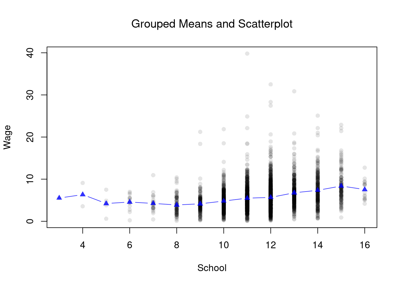
Scatterplots are a great and simplest plot for bivariate data that simply plots each observation. There are many extensions and similar tools. The example below helps understand how both the central tendency and dispersion change.
Code
# Running example for the whole chapter: wages and years of schooling
library(Ecdat)                              # provides Wages1
xy2_hat <- Wages1[order(Wages1[, 'school']), c('school', 'wage')]
colnames(xy2_hat) <- c('x_hat', 'y_hat') # x_hat=years of schooling, y_hat=hourly wage

# Scatter of every observation
plot(y_hat ~ x_hat, data=xy2_hat, pch=16, col=grey(0, .1),
    main=NA, xlab='School', ylab='Wage')

# Conditional mean at each integer schooling level
school_means <- aggregate(y_hat ~ x_hat, data=xy2_hat, mean)
points(y_hat ~ x_hat, data=school_means,    # connect dots so the trend pops
    pch=17, col=rgb(0, 0, 1, .8), type='b')
title('Grouped Means and Scatterplot', font.main=1)
Code
## Plot 2 (Alternative for big datasets)
# boxplot(y_hat ~ x_hat, data=xy2_hat,
#    pch=16, col=grey(0, .1), varwidth=T)
#title('Boxplots', font.main=1)

## Plot 3 (Less informative!)
#barplot(y_hat ~ x_hat, data=school_means)
#title('Bar Plot of Grouped Means', font.main=1)
Examine the local relationship between ‘Murder’ and ‘Urbanization’ in the USArrests dataset. Use custom bins.
Code
xy_hat <- USArrests[, c('UrbanPop', 'Murder')]
colnames(xy_hat) <- c('x_hat', 'y_hat') # x_hat=urban population share, y_hat=murder arrests per 100K
bins <- cut(xy_hat[, 'x_hat'], 6)
To move beyond descriptive statistics, we will use models. We previously covered linear models, but you could be analyzing data with nonlinear relationships. So now we consider a general relationship: \[
\hat{y}_{i} = M(\hat{x}_{i}) + \epsilon_{i},
\] where \(M\) is an unknown function and \(\epsilon_{i}\) is white noise, which we estimate via different models. After minimizing the sum of squared errors in the regressions below, our estimated models will also predict local averages.
Regressograms
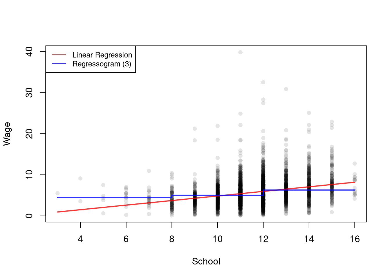
Just as a histogram summarizes how observations are distributed across bins of \(X\), a regressogram summarizes how the conditional mean of \(\hat{y}_{i}\) changes across bins of \(X\).
A regressogram splits \(X\) into exclusive intervals (bins) of half-width \(h\) and reports the average of \(\hat{y}_{i}\) within each bin.
The regressogram is useful when we expect the relationship between \(X\) and \(Y\) to bend in ways a single line cannot capture, because the bin averages can rise, fall, or stay flat from one bin to the next without imposing any global shape. It is the conditional-mean analog of a histogram: histograms count observations within bins of \(X\); regressograms average \(Y\) within bins of \(X\).
Code
# Data
plot(y_hat ~ x_hat, data=xy2_hat, pch=16, col=grey(0, .1),
    main=NA, xlab='School', ylab='Wage')
# xy2_hat defined above

## Simple Regression
reg  <- lm(y_hat ~ x_hat, data=xy2_hat) ## OLS

# Regressogram: Coarse Schooling Bins
xy2_hat[, 'xcc'] <- cut(xy2_hat[, 'x_hat'], 2)
rgram_c  <- lm(y_hat ~ xcc, data=xy2_hat)

# Regressogram: Fine Schooling Bins
xy2_hat[, 'xcf']   <- cut(xy2_hat[, 'x_hat'], 3)
rgram_f  <- lm(y_hat ~ xcf, data=xy2_hat)

# Regressogram (Means for each level)
xy2_hat[, 'xd']   <- as.factor(xy2_hat[, 'x_hat'])
rgram_d  <- lm(y_hat ~ xd, data=xy2_hat)

## Compare Models (Only 2 for simplicity)
lines( xy2_hat[, 'x_hat'], predict(reg), lwd=2, col=rgb(1, 0, 0, .8))
lines( xy2_hat[, 'x_hat'], predict(rgram_f), lwd=2, col=rgb(0, 0, 1, .8), type='s')
legend('topleft',
    legend=c('Linear Regression', 'Regressogram (3)'),
    col=c(rgb(1, 0, 0, .8), rgb(0, 0, 1, .8)),
    lty=1, cex=.8)
To conduct a regressogram, first divide \(X\) into \(1,...L\) exclusive bins of half-width \(h\). Each bin has a midpoint, \(x\), and each observation has an associated dummy variable \(\hat{d}_{i}(x,h) = \mathbf{1}\left(\hat{x}_{i}~\text{in}~\left(x-h,x+h\right] \right)\).
The half-width \(h\) controls how “local” a local estimate actually is.
The bandwidth \(h\) is the half-width of a local bin around the design point \(x\): an observation is “local” to \(x\) when \(|\hat{x}_{i}-x|\leq h\).
The bandwidth is useful as the central tuning knob for every local method in this chapter: regressograms, piecewise regression, locally constant kernel regression, and locally linear regression. It is the same \(h\) that set the bin half-width of a histogram and the spread of a kernel density, except that there it controlled how much data went into a density estimate at \(x\), and here it controls how much data goes into a conditional-mean estimate at \(x\). Larger \(h\) pools more observations into each estimate but smooths over real variation; smaller \(h\) tracks the data more closely but uses fewer points per estimate, so the fitted curve becomes noisier. Then we conduct a regression with this model: \[\begin{aligned}
\hat{y}_{i} &= \sum_{x~\text{in}~\{x_{1}, ..., x_{L} \}} b_{0}(x,h) \hat{d}_{i}(x,h) + \hat{e}_{i},
\end{aligned}\] where each bin has a coefficient \(b_{0}(x,h)\). Here \(\hat{e}_{i}\) depends on the trial bin coefficients \(b_{0}(x,h)\); the final residuals use the fitted coefficients \(\hat{b}_{0}(x,h)\).
Local Averages
When minimizing the sum of squared errors, the optimal coefficients are denoted as \(\hat{b}_{0}(x,h)\) and we can find them analytically. To do so, notice that each bin has \(n(x,h) = \sum_{i}^{n}\hat{d}_{i}(x,h)\) observations. This means we can split the dataset into parts associated with each bin \[\begin{aligned}
\sum_{i}^{n}\left[\hat{e}_{i}\right]^2
&= \sum_{i}^{n}\left[\hat{y}_{i}- \sum_{x~\text{in}~\{x_{1}, ..., x_{L} \}} b_{0}(x,h) \hat{d}_{i}(x,h) \right]^2 \\
&= \sum_{i}^{n(x_{1},h)}\left[\hat{y}_{i}- \sum_{x~\text{in}~\{x_{1}, ..., x_{L} \}} b_{0}(x,h) \hat{d}_{i}(x,h) \right]^2
+ ... \sum_{i}^{n(x_{L},h)}\left[\hat{y}_{i}- \sum_{x~\text{in}~\{x_{1}, ..., x_{L} \}} b_{0}(x,h) \hat{d}_{i}(x,h) \right]^2 \\
&= \sum_{i}^{n(x_{1},h)}\left[\hat{y}_{i}- b_{0}\left(x_1,h\right) \right]^2 + ... \sum_{i}^{n(x_L,h)}\left[\hat{y}_{i}-b_{0}\left(x_L,h\right) \right]^2 % +~ (N-1)\sum_{i}\hat{y}_{i}.
\end{aligned}\] This separation allows us to analytically optimize for each bin separately \[\begin{aligned}
\min_{ \left\{ b_{0}(x,h) \right\} } \sum_{i}^{n}\left[\hat{e}_{i}\right]^2
&= \min_{ \left\{ b_{0}(x,h) \right\} } \sum_{i}^{n(x,h)}\left[\hat{y}_{i}- b_{0}\left(x,h\right) \right]^2,
\end{aligned}\] In any case, minimizing yields the optimal coefficient as follows \[\begin{aligned}
0 &= -2 \sum_{i}^{n(x,h)}\left[ \hat{y}_{i} - b_{0}(x,h) \right] \\
\hat{b}_{0}(x,h) &= \frac{\sum_{i}^{n(x,h)} \hat{y}_{i}}{ n(x,h) } = \hat{m}_{Y}(x,h).
\end{aligned}\] As such, the OLS regression yields coefficients that are interpreted as the conditional mean: \(\hat{m}_{Y}(x,h)\). We can directly compute the same statistic directly by simply taking the average value of \(\hat{y}_{i}\) for all \(i\) observations in a particular bin.
In any case, the values predicted by the model are found as \[
\hat{y}_{i}^{\mathrm{fit}} = \sum_{x} \hat{b}_{0}(x,h) \hat{d}_{i}(x,h) = \sum_{x} \hat{m}_{Y}(x,h) \hat{d}_{i}(x,h).
\] I.e., the predicted value of observation \(i\) is the average value for its bin.
Consider this two-bin regressogram example of how schooling affects wage for people with \(\leq 9\) years of school completed vs \(> 9\). \[\begin{aligned}
\text{Wage}_{i} &= b_{0}(x=4.5, h=9/2) \mathbf{1}\left(\text{Educ}_{i}~\text{in}~(0,9]\right) + b_{0}(x=13.5, h=9/2) \mathbf{1}\left(\text{Educ}_{i}~\text{in}~(9,18] \right) + \hat{e}_{i}.
\end{aligned}\]
Here is a simple example with three data points \((\hat{x}_{i}, \hat{y}_{i})~\text{in}~\{ (1,2), (4,4), (12,3) \}\), we can easily compute \[\begin{aligned}
n(x=4.5,h=9/2) &= 2 \\
\hat{b}_{0}(x=4.5, h=9/2) &= [2 + 4] / 2 \\
n(x=13.5,h=9/2) &= 1 \\
\hat{b}_{0}(x=13.5, h=9/2) &= 3 / 1
\end{aligned}\]
Here is a simple example with data
Code
y_fit_c <- predict(rgram_c)
pred_dat <- data.frame(xcc=xy2_hat[, 'xcc'], y_fit=round(y_fit_c, 6))
table(pred_dat)
##             y_fit
## xcc          4.115873 5.917872
##   (2.99,9.5]      293        0
##   (9.5,16]          0     3001

## Compare to simple aggregation
aggregate(y_hat ~ xcc, data=xy2_hat, mean)
##          xcc    y_hat
## 1 (2.99,9.5] 4.115873
## 2   (9.5,16] 5.917872
Piecewise Regression
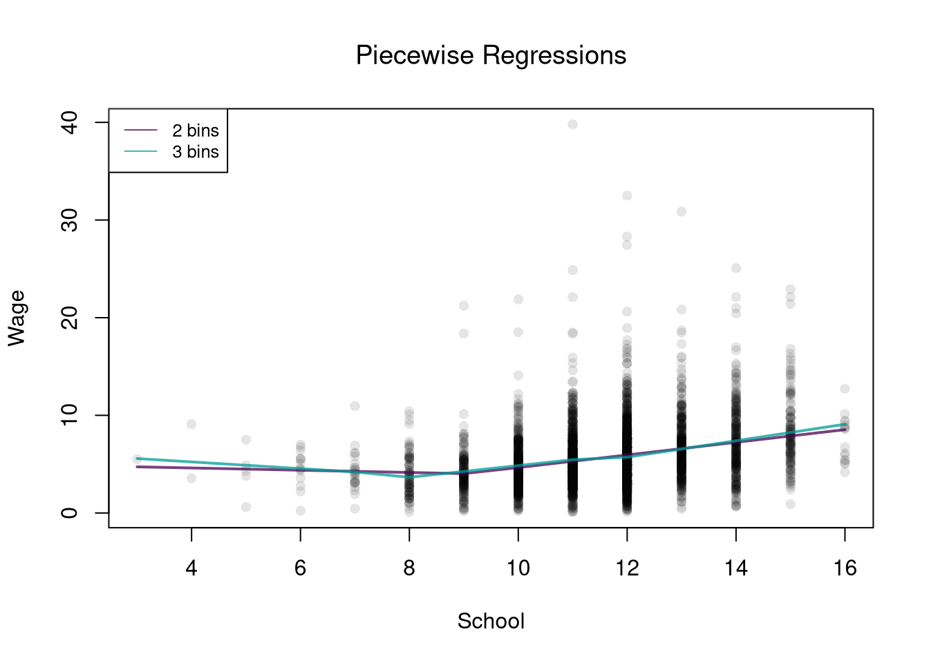
To let the slope vary across the range of \(X\) instead of just the level, we add a slope term within each bin.
A piecewise regression (also segmented regression) divides \(X\) into bins and runs a separate simple linear regression on each bin. Within a bin the relationship is a straight line; across bins the slope and intercept can change.
Piecewise regression is useful when the relationship is approximately linear in pieces but the slope itself changes. Returns to schooling might flatten after a degree, for example, or marginal cost curves might kink at capacity. Compared to the regressogram, it captures within-bin trends instead of just within-bin averages; compared to a single line, it lets the slope bend at bin boundaries.
Code
# Data
plot(y_hat ~ x_hat, data=xy2_hat, pch=16, col=grey(0, .1),
    main=NA, xlab='School', ylab='Wage')
# xy2_hat defined above

# Piecewise: Coarse Schooling Bins
xy2_hat[, 'xcc'] <- cut(xy2_hat[, 'x_hat'], 2)
preg_c  <- lm(y_hat ~ xcc*x_hat, data=xy2_hat)

# Piecewise: Fine Schooling Bins
xy2_hat[, 'xcf']   <- cut(xy2_hat[, 'x_hat'], 3)
preg_f  <- lm(y_hat ~ xcf*x_hat, data=xy2_hat)

## Compare Models
pw_cols <- hcl.colors(3, alpha=.75)
lines( xy2_hat[, 'x_hat'], predict(preg_c), lwd=2, col=pw_cols[1])
lines( xy2_hat[, 'x_hat'], predict(preg_f), lwd=2, col=pw_cols[2])
legend('topleft',
    legend=c('2 bins', '3 bins'),
    lty=1, col=pw_cols[1:2], cex=.8)
title('Piecewise Regressions', font.main=1)
The model is \[\begin{aligned}
\hat{y}_{i} &= \sum_{x} \left[b_{0}(x,h) + b_{1}(x,h)\hat{x}_{i} \right] \hat{d}_{i}(x,h) + \hat{e}_{i}.
\end{aligned}\] This same separation as above allows us to analytically optimize for each bin separately. I.e. we run separate regressions on the split samples. From the previous chapter on simple linear regression, we know the solutions are \[\begin{aligned}
\hat{b}_{0}(x,h) &= \hat{m}_{Y}(x,h)-\hat{b}_{1}\hat{m}_{X}(x,h) \\
\hat{b}_{1}(x,h) &= \frac{\sum_{i}^{n(x,h)}(\hat{x}_{i}-\hat{m}_{X}(x,h))(\hat{y}_{i}-\hat{m}_{Y}(x,h))}{\sum_{i}^{n(x,h)}(\hat{x}_{i}-\hat{m}_{X}(x,h))^2} = \frac{\hat{c}_{XY}(x,h)}{\hat{v}_{X}(x,h)},
\end{aligned}\]
Code
# See that two methods give the same predictions
# Piecewise: Coarse Schooling Bins
xy2_hat[, 'xcc'] <- cut(xy2_hat[, 'x_hat'], 2)
preg_c  <- lm(y_hat ~ xcc*x_hat, data=xy2_hat)
y_fit_piecewise <- predict(preg_c)

## Split Sample Regressions
xy2_split_hat <- split( xy2_hat, xy2_hat[, 'xcc'])
y_fit_split <- vector('list', length(xy2_split_hat))
names(y_fit_split) <- names(xy2_split_hat)
for (i in seq_along(xy2_split_hat)) {
    reg2 <- lm(y_hat ~ x_hat, xy2_split_hat[[i]])
    y_fit_split[[i]] <- predict(reg2)
}

# Any differences?
all( abs(y_fit_piecewise - unlist(y_fit_split)) < 1e-10 )
## [1] TRUE
Compare a simple regression to a regressogram and a piecewise regression. Examine the relationship between ‘Murder’ and ‘Urbanization’ in the USArrests dataset.
Code
xy_hat <- USArrests[, c('UrbanPop', 'Murder')]
colnames(xy_hat) <- c('x_hat', 'y_hat') # x_hat=urban population share, y_hat=murder arrests per 100K

# Globally Linear
reg <- lm(y_hat ~ x_hat, data=xy_hat)
Try to do so on your own before looking at the code below, which compares two piecewise regressions to a simple linear regression.
Code
# Diagnose Fit
#plot( fitted(reg), resid(reg), pch=16, col=grey(0, .5))
#plot( xy_hat[, 'x_hat'], resid(reg), pch=16, col=grey(0, .5))

# Linear in 2 Pieces (subsets)
xcut2 <- cut(xy_hat[, 'x_hat'], 2)
xy_list2 <- split(xy_hat, xcut2)
regs2 <- vector('list', length(xy_list2))
names(regs2) <- names(xy_list2)
for (i in seq_along(xy_list2)) {
    regs2[[i]] <- lm(y_hat ~ x_hat, data=xy_list2[[i]])
}

# Linear in 3 Pieces (subsets or bins)
xcut3 <- cut(xy_hat[, 'x_hat'], seq(32, 92, by=20), include.lowest=TRUE) # Finer Bins
xy_list3 <- split(xy_hat, xcut3)
regs3 <- vector('list', length(xy_list3))
names(regs3) <- names(xy_list3)
for (i in seq_along(xy_list3)) {
    regs3[[i]] <- lm(y_hat ~ x_hat, data=xy_list3[[i]])
}

## Make Predictions
pred1 <- data.frame(y_fit=predict(reg),
                    x_hat=reg[['model']][, 'x_hat'])
pred1 <- pred1[order(pred1[, 'x_hat']), ]

pred2 <- vector('list', length(regs2))
for (i in seq_along(regs2)) {
    pred2[[i]] <- data.frame(y_fit=predict(regs2[[i]]),
               x_hat=regs2[[i]][['model']][, 'x_hat'])
}
pred2 <- do.call(rbind, pred2)
pred2 <- pred2[order(pred2[, 'x_hat']), ]

pred3 <- vector('list', length(regs3))
for (i in seq_along(regs3)) {
    pred3[[i]] <- data.frame(y_fit=predict(regs3[[i]]),
               x_hat=regs3[[i]][['model']][, 'x_hat'])
}
pred3 <- do.call(rbind, pred3)
pred3 <- pred3[order(pred3[, 'x_hat']), ]

# Compare Predictions
plot(y_hat ~ x_hat, pch=16, col=grey(0, .5), data=xy_hat)
lines(y_fit ~ x_hat, pred1, lwd=2, col=2)
lines(y_fit ~ x_hat, pred2, lwd=2, col=4)
lines(y_fit ~ x_hat, pred3, lwd=2, col=3)
legend('topleft',
    legend=c('Globally Linear',
             'Piecewise Linear (2)',
             'Piecewise Linear (3)'),
    lty=1, col=c(2, 4, 3), cex=.8)
For many things, a simple linear regression, regressograms, or piecewise regression is “good enough”. Simple linear regressions struggle with nonlinear relationships but are very easy to run with a computer. Regressograms and piecewise regressions are intuitive ways to capture nonlinear relationships that are computationally efficient but have obvious problems where the bins change. Sometimes we want smoother predictions or to estimate derivatives (gradients). To cover more advanced regression methods that do those things, we will need to first learn about kernel density estimation.
Weighted Regression
Interestingly, we can obtain the same statistics from weighted least squares regression. For some specific design point, \(x\), we can find \(\hat{b}(x, h)\) by minimizing \[\begin{aligned}
\sum_{i}^{n}\left[ \hat{e}_{i} \right]^2 \hat{d}_{i}(x,h) &= \sum_{i}^{n}\left[ \hat{y}_{i}- b_{0}(x,h) - b_{1}(x,h) \hat{x}_{i} \right]^2 \hat{d}_{i}(x,h) \\
&= \sum_{i}^{n(x_{1},h)}\left[ \hat{y}_{i}- b_{0}(x_{1},h) - b_{1}(x_{1},h) \hat{x}_{i} \right]^2 \hat{d}_{i}(x_{1},h) + ... \sum_{i}^{n(x_{L},h)}\left[ \hat{y}_{i}- b_{0}(x_{L},h) - b_{1}(x_{L},h) \hat{x}_{i} \right]^2 \hat{d}_{i}(x_{L},h) \\
&= \sum_{i}^{n(x,h)}\left[\hat{y}_{i}- b_{0}\left(x,h\right) - b_{1}(x,h) \hat{x}_{i} \right]^2
\end{aligned}\]
We get nearly identical results if we instead use “uniform weights” with half-width \(h\), \[\begin{aligned}
k_{U}\left( \hat{x}_{i}, x, h \right)
&= \frac{\mathbf{1}\left(\frac{|\hat{x}_{i}-x|}{h} \leq 1\right)}{2}
= \frac{\mathbf{1}\left( \hat{x}_{i}~\text{in}~\left[ x-h, x + h\right] \right) }{2}
\end{aligned}\] which is nearly identical to \(\hat{d}_{i}(x,h)/ 2\), but uses intervals \([]\) instead of \((]\). As such we can see that \[\begin{aligned}
\sum_{i}^{n}\left[ \hat{e}_{i} \right]^2 k_{U}\left( \hat{x}_{i}, x, h \right)
&\approx \sum_{i}^{n}\left[ \hat{e}_{i} \right]^2 \hat{d}_{i}(x,h) / 2 \\
&= \sum_{i}^{n(x,h)}\left[\hat{y}_{i}- b_{0}\left(x,h\right) - b_{1}(x,h) \hat{x}_{i} \right]^2 / 2,
\end{aligned}\] The constant term \(1/2\) is irrelevant to finding the optimal solution (you can check the math yourself).
Here is the weighted regression on the wage data, at the midpoint of the first bin of the two-bin piecewise regression. Both predictions are the same, about \(4.551\).
Code
# xy2_hat defined above

## Weighted Regression
x <- 4.5 # regressogram bin1 midpoint
h <- 9.036/2 #window [-0.018, 9.018] covers schooling levels 3 to 9
k <- abs(xy2_hat[, 'x_hat']-x) /h
k_weights <- dunif(k, -1, 1) # the uniform kernel k_U
preg_k  <- lm(y_hat ~ x_hat, data=xy2_hat, weights=k_weights)
predict(preg_k, newdata=data.frame(x_hat=x))
##        1
## 4.551132

# Compare to Piecewise
xy2_hat[, 'xcc'] <- cut(xy2_hat[, 'x_hat'], 2)
preg_c  <- lm(y_hat ~ xcc*x_hat, data=xy2_hat)
predict(preg_c, newdata=data.frame(x_hat=x, xcc='(2.99,9.5]'))
##        1
## 4.551132
Check the same result at a different design point. Use the second bin, (9.5,16], which holds schooling levels \(10\) to \(16\).
Code
x <- 13 # middle of schooling levels 10 to 16
h <- 3 # uniform window [10, 16]

## Weighted Regression
k_weights <- dunif( abs(xy2_hat[, 'x_hat']-x)/h, -1, 1)
preg_k  <- lm(y_hat ~ x_hat, data=xy2_hat, weights=k_weights)
predict(preg_k, newdata=data.frame(x_hat=x))
##        1
## 6.592354

# Compare to Piecewise
predict(preg_c, newdata=data.frame(x_hat=x, xcc='(9.5,16]'))
##        1
## 6.592354
Here is an example going into the details of the weights.
Code
## Generate Sample Data
x0_hat <- 1:5
y0_hat <- round( rnorm(length(x0_hat)) , 2)
y0_hat
## [1] -0.26  0.10 -0.67  0.73  0.12
## plot(x0_hat, y0_hat)

## Manually Compute Estimate at x=3
h <- 1
k3_weights <- dunif( abs(x0_hat-3)/h, -1, 1) #(x0_hat >= 2)*(x0_hat <= 4)
k3_weights
## [1] 0.0 0.5 0.5 0.5 0.0

# Divide by the total so the weights sum to one
w3 <- k3_weights/sum(k3_weights)
y_fit_3 <- sum(w3*y0_hat)
y_fit_3
## [1] 0.05333333

# Equals the simple average of the y's within h of x=3
mean( y0_hat[ abs(x0_hat-3) <= h ] )
## [1] 0.05333333
Locally Constant Regression
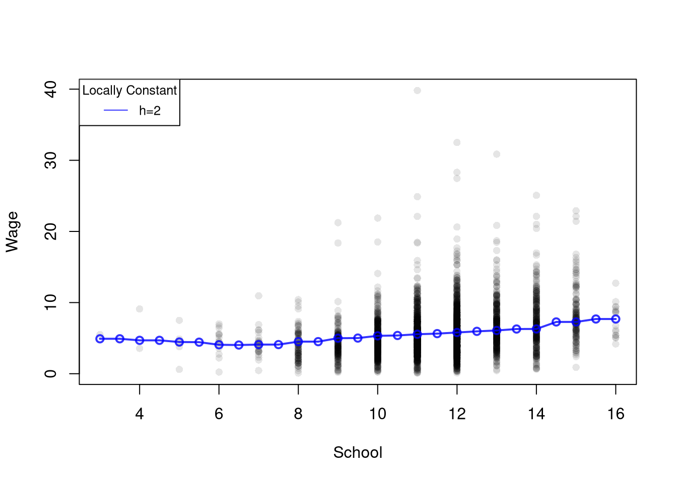
By replacing the hard bin indicator with a smooth kernel weight, we can fit a local average at every design point and get a curve that varies continuously with \(x\).
A locally constant (kernel) regression fits a single constant at each design point \(x\) by minimizing a kernel-weighted sum of squared residuals: \[\min_{b_{0}(x, h)} \sum_{i=1}^{n}\left[\hat{y}_{i} - b_{0}(x, h) \right]^{2} k\left(\hat{x}_{i}, x, h\right),\] where \(k(\hat{x}_{i}, x, h)\) is a kernel weight that down-weights observations far from \(x\).
The locally constant regression is useful as the simplest smoother that produces a continuous fitted curve: at each \(x\) it returns a kernel-weighted average of nearby \(\hat{y}_{i}\). With a uniform kernel and exclusive bins it reduces to a regressogram, so the regressogram is just its simplest special case.
For some intuition, consider a point \(x\) and the model \(\hat{y}_{i} = b_{0}(x, h) + \hat{e}_{i}\). The weighted OLS estimator with uniform kernel weights \(k_{U}\) yields \[\begin{aligned}
& \min_{b_{0}(x,h)}~ \sum_{i}^{n}\left[\hat{e}_{i} \right]^2 k_{U}\left( \hat{x}_{i}, x, h \right) \\
\Rightarrow & -2 \sum_{i}^{n}\left[\hat{y}_{i}- b_{0}(x, h) \right] k_{U}\left(\hat{x}_{i}, x, h\right) = 0 \\
\Rightarrow & \hat{b}_{0}(x)
= \frac{\sum_{i} \hat{y}_{i} k_{U} \left( \hat{x}_{i}, x, h \right) }{ \sum_{i} k_{U}\left( \hat{x}_{i}, x, h \right) }
= \sum_{i} \hat{y}_{i} \left[ \frac{ k_{U} \left( \hat{x}_{i}, x, h \right) }{ \sum_{i} k_{U}\left( \hat{x}_{i}, x, h \right)} \right]
= \sum_{i} \hat{y}_{i} w_{i}(x, h),
\end{aligned}\] where weights are determined from \[\begin{aligned}
\sum_{i}^{n} k_{U} \left( \hat{x}_{i}, x, h \right) &= \sum_{i}^{n(x,h)} k_{U} \left( \hat{x}_{i}, x, h \right) + \sum_{i}^{n - n(x,h)} 0 = \frac{n(x, h)}{2} \\
w_{i}(x, h) &= \left[ \frac{ k_{U} \left( \hat{x}_{i}, x, h \right) }{ \sum_{i} k_{U}\left( \hat{x}_{i}, x, h \right)} \right]
= \frac{\mathbf{1}\left( |\hat{x}_{i} - x| \leq h \right)}{n(x, h)}
\end{aligned}\] So locally constant kernel regression recovers the weighted mean of \(\hat{y}_{i}\) around design point \(x\). If we use exclusive bins, then we are essentially running a regressogram. As such, the regressogram is more crude but can be estimated more easily.
Here is the locally constant regression on the wage data. At each design point, we take the kernel-weighted average of wages for people with nearby years of schooling.
Code
# xy2_hat defined above
x_values <- seq(3, 16, by=.5) # Design points
h <- 2 # bandwidth

# Kernel-weighted mean at each design point
y_fit_lc <- rep(NA, length(x_values))
for (i in seq_along(x_values)) {
    ki <- dunif( abs(xy2_hat[, 'x_hat']-x_values[i])/h, -1, 1) # the uniform kernel k_U
    wi <- ki/sum(ki) # weights sum to one
    y_fit_lc[i] <- sum(wi*xy2_hat[, 'y_hat'])
}

# Plot
plot(y_hat ~ x_hat, data=xy2_hat, pch=16, col=grey(0, .1),
    main=NA, xlab='School', ylab='Wage')
lines(x_values, y_fit_lc, col=rgb(0, 0, 1, .8), lwd=2, type='o')
legend('topleft', title='Locally Constant',
    legend='h=2',
    lty=1, col=rgb(0, 0, 1, .8), cex=.8)
Notes
When \(n\) is small, \(\hat{b}_{U}(x, h)\) is typically estimated for each unique observed value: \(x~\text{in}~\{ x_{1},...x_{n} \}\). For large datasets, you can select a subset or evenly spaced values of \(x\) for which to make predictions.
If \(\hat{x}_{i}\) represents time, then the local constant regression is also called a moving average. We can create a weighted moving average by using a different distribution. I.e. using the Normal dnorm instead of the Uniform dunif.
The basic idea also generalizes other kernels. As such, a kernel regression using uniform weights is often called a “naive kernel regression”. Typically, kernel regressions use kernels that weight nearby observations more heavily.
Bias
The regressogram has a bias at the edges of the bins, which is addressed by the local constant regression. Still, the local constant regression has a bias near the edges of the dataset. (The kernel divides by \(2h\) assuming there is data on both sides of the design point). This can be addressed by renormalizing weights.
Here is an example going into the details of the weights.
Code
## Generate Sample Data
x0_hat <- 1:5
y0_hat <- rnorm(length(x0_hat))
y0_hat
## [1]  0.4323310 -0.1360990  0.3463146 -1.5691319 -1.0996329

## Manually Compute Estimate at x=5
h <- 2
k5_weights <- dunif( abs(x0_hat-5)/h, -1, 1) #(x0_hat >= 3)*(x0_hat =< 7)/2
k5_weights
## [1] 0.0 0.0 0.5 0.5 0.5

y_fit_5 <- sum(k5_weights*y0_hat)
y_fit_5
## [1] -1.161225

## Edge Correction
k5_weights_ec <- k5_weights/sum(k5_weights)
y_fit_5_ec <- sum(k5_weights_ec*y0_hat)
y_fit_5_ec
## [1] -0.7741501
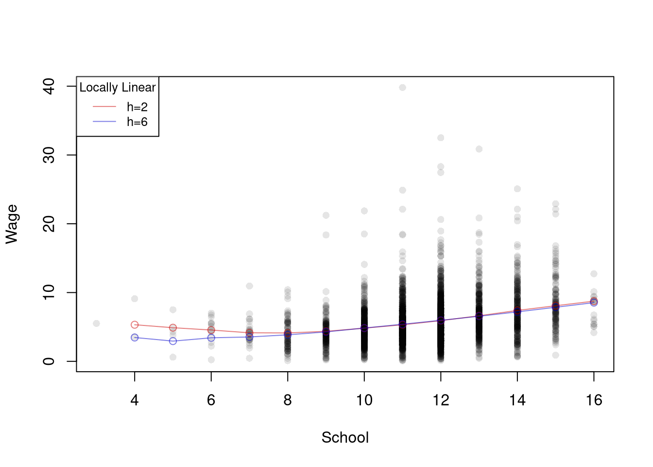
We can also add a slope term to address the bias.
Local Linear Regression
A less simple case is a local linear regression which conducts a linear regression for each data point using a subsample of data around it. Consider a point \(x\) and model \(\hat{y}_{i} = b_{0}(x,h) + b_{1}(x) \hat{x}_{i} + \hat{e}_{i}\) for data near \(x\). The weighted OLS estimator with kernel weights is \[\begin{aligned}
& \min_{b_{0}(x, h),b_{1}(x, h)}~ \sum_{i}^{n}\left[\hat{y}_{i}- b_{0}(x, h) - b_{1}(x,h) \hat{x}_{i} \right]^2 k_{U}\left( \hat{x}_{i}, x, h\right)
\end{aligned}\] Deriving the optimal values \(\hat{b}_{0}(x, h)\) and \(\hat{b}_{1}(x,h)\) for \(k_{U}\) is left as a homework exercise.
Code
# 'Naive' Smoother
pred_fun <- function(x0, h){
    # Assign equal weight to observations within h distance to x0
    # 0 weight for all other observations
    ki <- abs(xy2_hat[, 'x_hat']-x0)/h
    ki <- dunif(ki, -1, 1) ## The uniform kernel k_U; could change, e.g. dnorm(ki)
    wi <- ki/sum(ki, na.rm=TRUE) # always sum to 1 (for edge-effects)
    # run regression with weighted data
    llls_i <- lm(y_hat ~ x_hat, data=xy2_hat, weights=wi)
    y_fit <- predict(llls_i, newdata=data.frame(x_hat=x0))
}

x_values <- seq(4, 16, by=1) # Design points
# Fine Bins
y_fit_1 <- rep(NA, length(x_values))
for(i in seq_along(x_values)){
    y_fit_1[i] <- pred_fun(x0=x_values[i], h=2)
}
# Coarse Bins
y_fit_2 <- rep(NA, length(x_values))
for(i in seq_along(x_values)){
    y_fit_2[i] <- pred_fun(x0=x_values[i], h=6)
}

# Plot
plot(y_hat ~ x_hat, pch=16, data=xy2_hat, col=grey(0, .1),
    main=NA, ylab='Wage', xlab='School')
cols <- c(rgb(.8, 0, 0, .5), rgb(0, 0, .8, .5))
lines(x_values, y_fit_1, col=cols[1], lwd=1, type='o')
lines(x_values, y_fit_2, col=cols[2], lwd=1, type='o')
legend('topleft', title='Locally Linear',
    legend=c('h=2', 'h=6'),
    lty=1, col=cols, cex=.8)
Compare local linear and local constant regressions using https://shinyserv.es/shiny/kreg/, with degree \(0\) and \(1\). Also try different kernels and different datasets.
Examine the local relationship between ‘Murder’ and ‘Urbanization’ in the USArrests dataset using LLLS.
Code
# xy_hat defined above
# Same smoother as pred_fun, but for any data with columns x_hat and y_hat
pred_fun_xy <- function(x0, h, xy){
    ki <- abs(xy[, 'x_hat']-x0)/h
    ki <- dunif(ki, -1, 1) ## The uniform kernel k_U
    wi <- ki/sum(ki, na.rm=TRUE)
    llls_i <- lm(y_hat ~ x_hat, data=xy, weights=wi)
    y_fit <- predict(llls_i, newdata=data.frame(x_hat=x0))
}

x_values <- sort(unique(xy_hat[, 'x_hat']))
plot(y_hat ~ x_hat, pch=16, data=xy_hat, col=grey(0, .5),
    ylab='Murder Rate', xlab='Urban Population (%)')

y_fit_1 <- numeric(length(x_values))
for (i in seq_along(x_values)) {
    y_fit_1[i] <- pred_fun_xy(x_values[i], h=2, xy=xy_hat)
}

y_fit_2 <- numeric(length(x_values))
for (i in seq_along(x_values)) {
    y_fit_2[i] <- pred_fun_xy(x_values[i], h=20, xy=xy_hat)
}

cols <- c(rgb(.8, 0, 0, .5), rgb(0, 0, .8, .5))
lines(x_values, y_fit_1, col=cols[1], lwd=1, type='o')
lines(x_values, y_fit_2, col=cols[2], lwd=1, type='o')
legend('topleft', title='Locally Linear',
    legend=c('h=2 ', 'h=20'),
    lty=1, col=cols, cex=.8)
Exercises
Comment the script you wrote for this chapter, then restart R and check that it runs from a clean session, then check the script with AI as explained in Working with AI. Write three sentences from memory on the main statistical idea of this chapter, and ask the assistant what is wrong, vague, or missing. Finish with your own questions about whatever you found hardest.
Explain the difference between a regressogram and a local linear regression. As you increase the number of bins in a regressogram, what happens to the number of observations in each bin, and how does that change the fitted values?
Using the Wages1 dataset from the Ecdat package, fit a regressogram with 4 bins and a piecewise regression with 4 bins for the relationship between wage and school. Compute the predicted value at school = 10 for each model.
Using the USArrests dataset, write R code to estimate a local linear regression of Murder on UrbanPop using uniform kernel weights with bandwidth \(h = 10\). Compute predictions at design points x_values <- seq(40, 80, by = 10) and plot them over the scatterplot.
The chapter derives the optimal locally constant coefficient \(\hat{b}_{0}(x,h)\) but leaves the local linear case as an exercise. Starting from the weighted objective \(\sum_{i} [\hat{y}_{i} - b_{0} - b_{1}\hat{x}_{i}]^2 \, k_{U}(\hat{x}_{i}, x, h)\), set the partial derivatives with respect to \(b_{0}\) and \(b_{1}\) to zero. Show that the solution is the simple-regression formula applied to the kernel-weighted data: \(\hat{b}_{1}(x,h) = \hat{c}_{XY}(x,h)/\hat{v}_{X}(x,h)\) and \(\hat{b}_{0}(x,h) = \hat{m}_{Y}(x,h) - \hat{b}_{1}(x,h)\hat{m}_{X}(x,h)\).
Recall
This chapter let the wage-schooling relationship bend by fitting local models on the Wages1 data: regressograms (bin means), piecewise regression (bin lines), locally constant kernel regression, and locally linear regression. The three-observation worked example \(\{(1, 2), (4, 4), (12, 3)\}\) split into two bins at \(h=9/2\) gave regressogram coefficients \(\hat{b}_{0}(x=4.5)=(2+4)/2=3\) and \(\hat{b}_{0}(x=13.5)=3\).