9 Advanced Probability

9.1 Discrete Factorial Distributions

Binomial.

The sum of $n$ Bernoulli’s (number of successes) in $n$ trials.

\[\begin{eqnarray} X_{i} \in \{0,1,\ldots,n\} \\ Prob(X_{i}=x) &=& \binom{n}{x}p^{x}(1-p)^{n-x} \\ F(x) = Prob(X_{i} \leq x) &=& \sum_{k=0}^{\lfloor x \rfloor} Prob(X_{i}=x) \end{eqnarray}\]

The simplest case: how many heads will I get when I flip a fair coin twice? We can first see that there are four potential outcomes: $\{ (1,1), (1,0), (0,1), (0,0) \}$, each of which are equally likely. The corresponding sums of $\{2,1,1,0\}$ are equally likely, which leads to probabilities $Prob(X_{i}=0)=1/4$, $Prob(X_{i}=1)=2/4$, and $Prob(X_{i}=2)=1/4$.

If the coin is unfair; probability of heads equals $0.25$, then the corresponding outcomes $\{2,1,1,0\}$ have probability

Test Yourself

When I flip a coin three times, the potential outcomes are \[\begin{eqnarray} \{ (1,1,1), (1,1,0), (1,0,1), (1,0,0),\\ (0,1,1), (0,1,0), (0,0,1), (0,0,0) \} \end{eqnarray}\] Assuming the coin is fair, compute the probabilities for each possible sum. Assuming the coin is unfair, with probability of heads equal to $0.25$, compute the probabilities for each possible sum.

In general, we use the Binomial distribution. The $\binom{n}{x}$ term is called the binomial coefficient and it counts all the different groups lead to the same sum. The other terms intuitively reflect the probabilities of getting $x$ success and $n-x$ failures.

For example, suppose $n=15$ people walk past a store each hour and each has a $p=30\%$ chance of entering. The number of customers who enter is $X_{i} \sim \text{Binom}(15, 0.3)$.

Code

## Store: 15 passers-by, 30% chance each enters
n <- 15
p <- 0.3

# PMF plot
x <- seq(0, n)
f_x <- dbinom(x, n, p)
plot(x, f_x, type = 'h', col = rgb(0, 0, 1, .8),
    main=NA, xlab = 'Customers entering', ylab = 'Prob(X = x)')
title(bquote(paste('Binom(', .(n), ', ', .(p), ')')), font.main=1)
points(x, f_x, pch = 16, col = rgb(0, 0, 1, .8))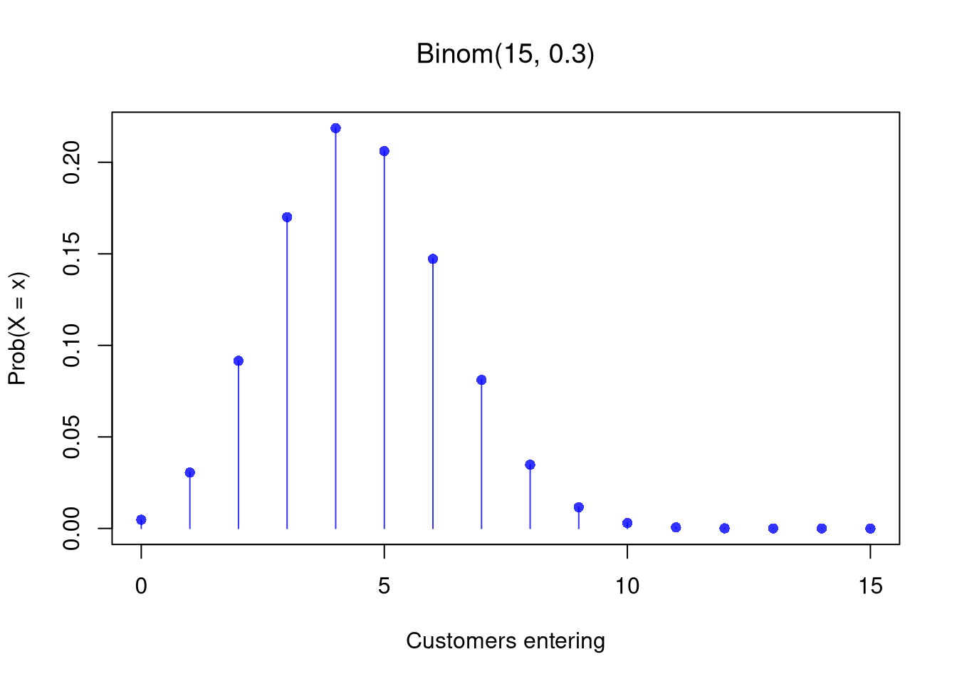

Code


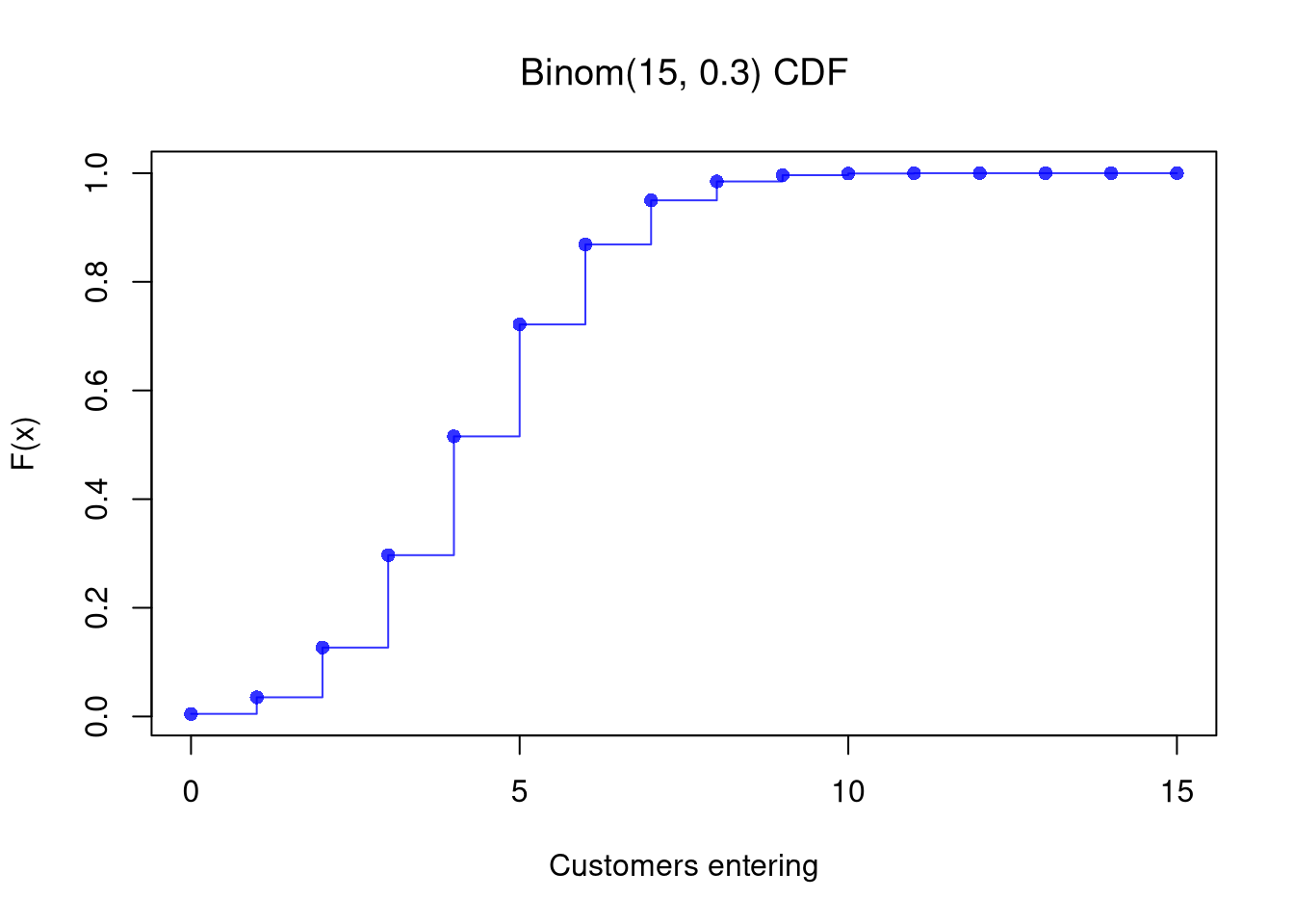
## Theoretical CDF
F_x <- pbinom(x, n, p)
plot(x, F_x, type='s', col=rgb(0, 0, 1, .8),
    xlab = 'Customers entering', ylab = 'F(x)', main=NA)
points(x, F_x, pch=16, col=rgb(0, 0, 1, .8))
title(bquote(paste('Binom(', .(n), ', ', .(p), ') CDF')), font.main=1)

Must Know

A quality inspector checks $n=20$ items from a production line with a $5\%$ defect rate ($p=0.05$). What is the probability of finding $2$ or fewer defectives?

We need $Prob(X_{i} \leq 2) = F(2)$ where $X_{i} \sim \text{Binom}(20, 0.05)$. By hand, the first few terms are \[\begin{eqnarray} Prob(X_{i}=0) &=& \binom{20}{0}(0.05)^{0}(0.95)^{20} \approx 0.36 \\ Prob(X_{i}=1) &=& \binom{20}{1}(0.05)^{1}(0.95)^{19} \approx 0.38 \\ Prob(X_{i}=2) &=& \binom{20}{2}(0.05)^{2}(0.95)^{18} \approx 0.19 \end{eqnarray}\] So $Prob(X_{i} \leq 2) \approx 0.36 + 0.38 + 0.19 = 0.93$. There is roughly a $93\%$ chance the inspector finds $2$ or fewer defectives.

Code

# Individual terms
x <- c(0, 1, 2)
px <- dbinom(x, size=20, prob=0.05)
round(px, 2)
## [1] 0.36 0.38 0.19

# CDF: Prob(X <= 2)
pbinom(2, size=20, prob=0.05)
## [1] 0.9245163

Test Yourself

Suppose that employees at a company are $70%$ female and $30%$ male. If we select a random sample of eight employees, what is the probability that $2$ in the sample are female? That $\geq 2$ are female?

Try conducting a simulation first,

Code

n <- 8
p <- 0.3
X <- rbinom(1000, n, p)

Test Yourself

For $n$ coin flips, show that $\mathbb{E}[X_{i}]=np$ and $\mathbb{V}[X_{i}]=np(1-p)$. Build on the case $n=2$ above, then consider case $n=3$, and then the general case of any $n$.

Code

# Compare empirical simulation vs theoretical
n <- 2
p <- 3/4
X <-  rbinom(1000, size=n, prob=p)

# Mean
c(empirical = mean(X), theoretical = n*p)
##   empirical theoretical 
##       1.483       1.500

# Variance
c(empirical  = var(X),  theoretical  = n*p*(1-p))
##   empirical theoretical 
##   0.4081191   0.3750000

Poisson.

The Poisson distribution models how many events occur in a fixed interval, when each individual event is rare and independent and has equal probabilities at any point on the interval.

In general, the Poisson distribution gives \[\begin{eqnarray} X_{i} \in \{0,1,\ldots\} \\ Prob(X_{i}=x) &=& e^{-\lambda}\lambda^x/x! \\ F(x) = Prob(X_{i} \leq x) &=& \sum_{k=0}^{\lfloor x \rfloor} Prob(X_{i}=x) \end{eqnarray}\] The single parameter $\lambda$ is the average number of events per interval. Note the infinite discrete support $\{0,1,2,\ldots\}$: there is no upper bound on the count, though large values become vanishingly unlikely.

For example, a small store averages $\lambda = 3.5$ customers per hour. In any given hour the actual count might be 2, or 5, or 7. For our store, $\lambda = 3.5$ means we expect 3.5 customers per hour on average and the following assumptions hold

Arrivals are independent of each other (one customer entering does not make the next more or less likely)
The average rate $\lambda$ is constant over the interval
Two customers cannot arrive at exactly the same instant

We can then compute a few probabilities by hand.E.g, the chance that zero customers arrive in a given hour is \[\begin{eqnarray} Prob(X_{i}=0) &=& e^{-3.5} \cdot 3.5^{0} / 0! = e^{-3.5} \approx 0.030 \end{eqnarray}\] The chance of exactly 2 customers is \[\begin{eqnarray} Prob(X_{i}=2) &=& e^{-3.5} \cdot 3.5^{2} / 2! = e^{-3.5} \cdot 6.125 \approx 0.185 \end{eqnarray}\]

Code

## Store: lambda = 3.5 customers per hour
lambda <- 3.5

# PMF plot
x <- seq(0, 15)
f_x <- dpois(x, lambda)
plot(x, f_x, type='h', col=rgb(0, 0, 1, .8),
     xlab = 'Customers per hour', ylab = 'Prob(X = x)', main=NA)
points(x, f_x, pch = 16, col = rgb(0, 0, 1, .8))
title(bquote(paste('Pois(', .(lambda), ')')), font.main=1)

Code


# CDF plot
F_x <- ppois(x, lambda)
plot(x, F_x, type='s', col=rgb(0, 0, 1, .8),
    xlab = 'Customers per hour', ylab = 'F(x)', main=NA)
points(x, F_x, pch=16, col=rgb(0, 0, 1, .8))
title(bquote(paste('Pois(', .(lambda), ') CDF')), font.main=1)

Test Yourself

Show that $\mathbb{E}[X_{i}] = \mathbb{V}[X_{i}]= \lambda$. That is, the Poisson mean and variance are both equal to the rate parameter.

Code

# Compare empirical simulation vs theoretical
lambda <- 3.5
X <- rpois(1e4, lambda)
c(emp_mean = mean(X), th_mean = lambda)
## emp_mean  th_mean 
##   3.5007   3.5000
c(emp_var  = var(X),  th_var  = lambda)
##  emp_var   th_var 
## 3.532153 3.500000

Must Know

During the lunch rush, the store averages $\lambda=4.5$ customers per hour. What is the probability that more than $7$ customers arrive in a given hour?

We need $Prob(X_{i} > 7) = 1 - Prob(X_{i} \leq 7) = 1 - F(7)$. \[\begin{eqnarray} Prob(X_{i} > 7) &=& 1 - \sum_{k=0}^{7} \frac{e^{-4.5} \cdot 4.5^{k}}{k!} \end{eqnarray}\]

Code

# Prob(X > 7)
1 - ppois(7, lambda=4.5)
## [1] 0.08658647

# Verify: sum the PMF from 0 to 7
sum(dpois(0:7, lambda=4.5))
## [1] 0.9134135

There is roughly a $9\%$ chance of more than $7$ arrivals in a given hour.

The shape of the Poisson also changes with $\lambda$. A quiet specialty shop ($\lambda=1$) has a strongly right-skewed arrival pattern, while a busy supermarket ($\lambda=15$) looks nearly Normal.

Code

# Shape varies with lambda
par(mfrow=c(1, 3))
for(lam in c(1, 5, 15)) {
    x <- seq(0, 30)
    f_x <- dpois(x, lam)
    plot(x, f_x, type='h', col=rgb(0, 0, 1, .8),
        xlab = 'Customers per hour', ylab = 'Prob(X = x)', main=NA)
    points(x, f_x, pch=16, col=rgb(0, 0, 1, .8))
    title(bquote(paste('Pois(', .(lam), ')')), font.main=1)
}

Large Sample Approximations.

The de Moivre–Laplace Theorem says that as $n$ grows large, with $p \in (0,1)$ staying fixed, the Binomial distribution is approximately Normal with mean $np$ and variance $np(1-p)$

Test Yourself

The unemployment rate is $10%$. Suppose that $100$ employable people are selected randomly. What is the probability that this sample contains between $9$ and $12$ unemployed people. Use the normal approximation to binomial probabilities.

Parameters are \[\begin{eqnarray} \mu &\approx& n p = 10 \\ \sigma^2 &=& n p (1−p) = 100 (0.1)(0.9)=9 \\ \sigma &=& \sqrt{9}=3. \end{eqnarray}\]

The Poisson Limit Theorem says that as $n$ grows large, with $p$ growing smaller at the same time, and $n p$ converging to a fixed number $\lambda$, the Binomial distribution is approximately Poisson with parameter $\lambda$.

Test Yourself

Imagine dividing one hour into $n$ tiny intervals. If the store averages $\lambda = 3.5$ customers per hour, each interval has a small probability $p = \lambda/n = 3.5/n$ of an arrival. With $n$ independent intervals, the number of arrivals is Binomial: \[Prob(X=x) = \binom{n}{x} \left(\frac{\lambda}{n}\right)^{x} \left(1-\frac{\lambda}{n}\right)^{n-x}\]

As $n$ grows large, three things happen:

$\binom{n}{x} \cdot \frac{1}{n^{x}} \to \frac{1}{x!}$, because $\binom{n}{x} = \frac{n(n-1)\cdots(n-x+1)}{x!}$ and each factor in the numerator is approximately $n$
$\left(1 - \frac{\lambda}{n}\right)^{n} \to e^{-\lambda}$, by the definition of $e$
$\left(1 - \frac{\lambda}{n}\right)^{-x} \to 1$, since $x$ is fixed and $\lambda/n \to 0$

Multiplying the pieces together: $\frac{1}{x!} \cdot \lambda^{x} \cdot e^{-\lambda} = e^{-\lambda}\lambda^{x}/x!$, which is the Poisson PMF. In other words, the Poisson is what the Binomial becomes when there are many opportunities for an event but each one is individually unlikely (see also Large Sample Approximations below).

Code

# Binomial approaches Poisson as n grows
lambda <- 3.5
x <- seq(0, 12)
f_pois <- dpois(x, lambda)

par(mfrow=c(1, 3))
for(n in c(10, 50, 1000)) {
    f_binom <- dbinom(x, size=n, prob=lambda/n)
    comp_cols <- c(rgb(.8, 0, 0, .5), rgb(0, 0, .8, .5))
    plot(x, f_binom, type='h', col=comp_cols[1], lwd=4,
        xlab='Customers', ylab='Prob(X = x)', main=NA)
    points(x + 0.2, f_pois, type='h', col=comp_cols[2], lwd=2)
    points(x + 0.2, f_pois, pch=16, col=comp_cols[2], cex=0.7)
    title(bquote(paste('Binom(', .(n), ', ', .(round(lambda/n, 4)), ')')), font.main=1)
}
legend('topright', c('Binomial', 'Poisson'),
    col=comp_cols, lwd=c(4, 2), cex=0.8)

Test Yourself

For another example, consider $n=1000$ independent trials each with probability $p=0.004$, so $\lambda = np = 4$. We can compare the exact Binomial to both approximations at once: the Poisson ($\lambda=4$) and the Normal ($\mu=np=4$, $\sigma^{2}=np(1-p)\approx 3.98$).

Code

# Binom(1000, 0.004) vs Pois(4) vs Normal(4, 3.98)
n <- 1000
p <- 0.004
x <- seq(0, 15)
f_binom <- dbinom(x, size=n, prob=p)
f_pois  <- dpois(x, lambda=n*p)
f_norm  <- dnorm(x, mean=n*p, sd=sqrt(n*p*(1-p)))

approx_cols <- hcl.colors(3, alpha=.45)
plot(x, f_binom, type='h', col=approx_cols[1], lwd=4,
    xlab='x', ylab='Prob(X = x)',
    main=NA)
title('Approximating the Binomial', font.main=1)
points(x + 0.15, f_pois, type='h', col=approx_cols[2], lwd=2)
lines(x, f_norm, col=approx_cols[3], lwd=2)
legend('topright',
    c('Binom(1000, 0.004)', 'Pois(4)', 'Normal(4, 3.98)'),
    col=approx_cols, lwd=c(4, 2, 2))

The Poisson is nearly exact here because $p$ is very small. The Normal is a rougher fit because $\lambda=4$ is still fairly small and the distribution is noticeably skewed. As $\lambda$ grows, the Poisson itself becomes more symmetric and the Normal approximation improves.

9.2 Continuous Factorial Distributions

Irwin–Hall.

Suppose the store has a tip jar and each customer drops in a random amount between $\$0$ and $\$1$. If $n=2$ customers visit, the total tips are the sum of two independent $\text{Uniform}(0,1)$ random variables. The Irwin-Hall distribution describes this sum for any $n$.

The support is continuous on $[0,n]$ and the probability density function is \[f(x) = \dfrac{1}{(n-1)!} \displaystyle\sum_{k=0}^{\lfloor x \rfloor} (-1)^k \binom{n}{k} (x - k)^{n-1}\] for $x \in [0,n]$, and $0$ otherwise. The parameter $n$ is the number of independent uniform contributions. When $n=1$ this is just the Uniform density; when $n=2$ it is a triangle peaking at $1$.

Code

## Tip jar: total tips from n customers, each Uniform(0, 1)
# Irwin-Hall PDF function
dirwinhall <- function(x, n) {
    f_x <- rep(NA, length(x))
    for(i in seq(x)) {
        xx <- x[i]
        if(xx < 0 | xx > n){
            f_x[i] <- 0
        } else {
            k <- seq(0, floor(xx))
            f_k <- sum((-1)^k*choose(n, k)*(xx-k)^(n-1))/factorial(n-1)
            f_x[i] <- f_k
        }
    }
    return(f_x)
}

# Two customers
n <- 2
x <- seq(0, n, length.out = 500)

# Compute and plot PDF
f_x <- dirwinhall(x, n)
plot(x, f_x, type='l', col=rgb(0, 0, 1, .8),
    main=NA, xlab = 'Total tips ($)', ylab = 'f(x)')
title(bquote(paste('IrwinHall(', .(n), ')')), font.main=1)

See also the Bates distribution, which is for the mean of $n$ i.i.d. $\text{Uniform}(0,1)$ random variables. It essentially rescales the Irwin-Hall distribution to range between $0$ and $1$.

Beta.

The fraction of customers who make a purchase varies from day to day. Some days 80% buy something; other days only 30%. The Beta distribution models this kind of proportion: a random variable on the unit interval $X_{i} \in [0,1]$ with flexible shape.

The Beta has two shape parameters. When both equal 2, the distribution is symmetric and bell-shaped on $[0,1]$, centering the purchase rate around $50\%$. The density formula is mathematically involved, so we omit it and work graphically instead.

Code

## Daily purchase rate: Beta(2, 2)
X4 <- rbeta(2000, 2, 2)
hist(X4, breaks=20, border=NA, main=NA, freq=F,
    xlab='Purchase rate')

x <- seq(0, 1, by=.01)
fx <- dbeta(x, 2, 2)
lines(x, fx, col=rgb(0, 0, 1, .8))

We can find probabilities using either the density (area under the curve) or the CDF.

Test Yourself

What is the probability that the daily purchase rate falls between $20\%$ and $80\%$? Intuitively depict this as the area under the density. Then compute it numerically using the CDF.

Code

plot(ecdf(X4), main=NA,
    xlab='Purchase rate') # Empirical

x <- seq(0, 1, by=.01) # Theoretical
Fx <- pbeta(x, 2, 2)
lines(x, Fx, col=rgb(0, 0, 1, .8))

# Middle Interval Example
F2 <- pbeta(0.2, 2, 2)
F8 <- pbeta(0.8, 2, 2)
F_2_8 <- F8 - F2
F_2_8
## [1] 0.792

# Visualize
title('Purchase rate between 0.2 and 0.8', font.main=1)
segments(0.2, F2, -1, F2, col=rgb(1, 0, 0, .8))
segments(0.8, F8, -1, F8, col=rgb(1, 0, 0, .8))

The two shape parameters allow the Beta to take many different shapes, making it useful whenever the quantity of interest is a proportion.

Test Yourself

Different shape parameters represent different beliefs about the store’s purchase rate. For each density below, intuitively depict $Prob(X_{i} \leq 0.5)$ using the PDF. Repeat the exercise using a CDF instead of a PDF to calculate a numerical value.

Code

op <- par(no.readonly = TRUE); on.exit(par(op), add = TRUE)
x <- seq(0, 1, by=.01)
pars <- expand.grid(c(.5, 1, 2), c(.5, 1, 2))
par(mfrow=c(3, 3))
apply(pars, 1, function(p){
    fx <- dbeta(x, p[1], p[2])
    plot(x, fx, type='l', xlim=c(0, 1), ylim=c(0, 4), lwd=2, col=rgb(0, 0, 1, .8),
        xlab='Purchase rate', ylab='f(x)', main=NA)
})
title('Beta densities', outer=T, line=-1, font.main=1)

9.3 Set Theory

Let the sample space contain events $A$ and $B$, with their probability denoted as $Prob(A)$ and $Prob(B)$. Then

the union: $A\cup B$, refers to either event occurring
the intersection: $A\cap B$, refers to both events occurring
the events $A$ and $B$ are mutually exclusive if and only if $A\cap B$ is empty
the inclusion–exclusion rule is: $Prob(A\cup B)=Prob(A)+Prob(B)-Prob(A\cap B)$
the events $A$ and $B$ are mutually independent if and only if $Prob(A\cap B)=Prob(A) Prob(B)$
the conditional probability is $Prob(A \mid B) = Prob(A \cap B)/ P(B)$

For example, consider a six sided die where events are the number $>2$ or the number is even.

The sets are $A=\{3,4,5,6\}$ and $B=\{2,4,6\}$
To check mutually exclusive: notice $A\cap B=\{4,6\}$ which is not empty. So event $A$ and event $B$ are not mutually exclusive

Further assuming the die are fair, each side has an equal $1/6$ probability. This lets us compute

$Prob(A)=4/6=2/3$ and $Prob(B)=3/6=1/2$
$A\cup B=\{2,3,4,5,6\}$, which implies $Prob(A\cup B)=5/6$
$A\cap B=\{4,6\}$, which implies $Prob(A\cap B)=2/6=1/3$
To check independence: notice $Prob(A\cap B)=1/3 = (2/3) (1/2) = Prob(A)Prob(B)$. So event $A$ and event $B$ are mutually independent
To check inclusion–exclusion: notice $Prob(A) + Prob(B) - Prob(A\cap B) = 2/3 + 1/2 - 1/3 = 4/6 + 3/6 - 2/6 = 5/6 = Prob(A\cup B)$
Finally, the conditional probability of $Prob(\text{die is} >2 \mid \text{die shows even number}) = Prob(A \mid B) = \frac{Prob(A \cap B)}{P(B)} = \frac{1/3}{1/2} = 2/3$

Code

# Simulation verification
set.seed(123)
x <- seq(1, 6)
rolls <- sample(x, 1e6, replace = TRUE)
A <- rolls > 2
B <- rolls %% 2 == 0
P_AcondB <- mean(A & B) / mean(B)
round(P_AcondB, 3)
## [1] 0.667

Test Yourself

Consider a six sided die with sample space $\{1,2,3,4,5,6\}$ where each outcome is each equally likely. What is $Prob(\text{die is odd or }<5)$? Denote the odd events as $A=\{1,3,5\}$ and the less than five events as $B=\{1,2,3,4\}$. Then

$A\cap B=\{1,3\}$, which implies $Prob(A\cap B)=2/6=1/3$.
$Prob(A)=3/6=1/2$ and $Prob(B)=4/6=2/3$.
By inclusion–exclusion: $Prob(A\cup B)=Prob(A)+Prob(B)-Prob(A\cap B)=1/2+2/3-1/3=5/6$.

Now find $Prob(\text{die is even and }<5)$. Verify your answer with a computer simulation.

Bayes’ Theorem.

Bayes’ theorem reverses the direction of a conditional probability. From the definition, $Prob(A \cap B) = Prob(B \mid A) \cdot Prob(A)$. Substituting into $Prob(A \mid B) = Prob(A \cap B) / Prob(B)$ gives \[\begin{eqnarray} Prob(A \mid B) &=& \frac{Prob(B \mid A) \cdot Prob(A)}{Prob(B)} \end{eqnarray}\]

In the die example above, we computed $Prob(A \mid B) = 2/3$: the probability the die is $>2$, given it is even. We can use Bayes’ theorem to reverse this: what is the probability the die is even, given it is $>2$?

Must Know

Using the same die with $A=\{3,4,5,6\}$ and $B=\{2,4,6\}$, we know $Prob(A \mid B)=2/3$, $Prob(B)=1/2$, and $Prob(A)=2/3$. By Bayes’ theorem, \[\begin{eqnarray} Prob(B \mid A) &=& \frac{Prob(A \mid B) \cdot Prob(B)}{Prob(A)} = \frac{(2/3)(1/2)}{2/3} = \frac{1}{2}. \end{eqnarray}\] We can verify directly: given $A=\{3,4,5,6\}$, the even outcomes are $\{4,6\}$, so $Prob(B \mid A)=2/4=1/2$. Since $A$ and $B$ are independent, $Prob(B \mid A) = Prob(B)$ and flipping the conditioning changes nothing.

Code

# Simulation verification
set.seed(123)
rolls <- sample(seq(1, 6), 1e6, replace=TRUE)
A <- rolls > 2
B <- rolls %% 2 == 0
# Prob(B | A)
mean(B[A])
## [1] 0.5001065

Bayes’ theorem is most useful when events are not independent, so that knowing $B$ occurred changes what we believe about $A$.

Test Yourself

A company sources parts from two suppliers. Supplier $A$ provides $60\%$ of parts and supplier $B$ provides $40\%$. The defect rate from supplier $A$ is $3\%$ and from supplier $B$ is $5\%$. If a randomly selected part is defective ($D$), what is the probability it came from supplier $A$?

We know $Prob(A)=0.6$, $Prob(\lnot A)=0.4$, $Prob(D \mid A)=0.03$, and $Prob(D \mid \lnot A)=0.05$. By the Law of Total Probability, \[\begin{eqnarray} Prob(D) &=& Prob(D \mid A) \cdot Prob(A) + Prob(D \mid \lnot A) \cdot Prob(\lnot A) \\ &=& 0.03 \times 0.6 + 0.05 \times 0.4 = 0.038. \end{eqnarray}\] By Bayes’ theorem, \[\begin{eqnarray} Prob(A \mid D) &=& \frac{Prob(D \mid A) \cdot Prob(A)}{Prob(D)} = \frac{0.03 \times 0.6}{0.038} \approx 0.474. \end{eqnarray}\] Even though supplier $A$ provides $60\%$ of all parts, they account for only about $47\%$ of defectives because their defect rate is lower.

Code

# Simulation verification
set.seed(42)
n <- 1e6
supplier <- sample(c('A', 'B'), n, replace=TRUE, prob=c(0.6, 0.4))
defect_rate <- ifelse(supplier == 'A', 0.03, 0.05)
defective <- runif(n) < defect_rate

# Prob(A | D)
mean(supplier[defective] == 'A')
## [1] 0.4796915

Law of Total Probability.

This law states that $Prob(A)=Prob(A \mid B) P(B) + Prob(A \mid \lnot B) P(\lnot B)$, where $\lnot B$ is the event “not $B$”.

For example, consider a six sided die where events are the number $>2$ or the number is even. - The sets are $A=\{3,4,5,6\}$ and $B=\{2,4,6\}$ and $\lnot B = \{1,3,5\}$ From before, we know that $Prob(A)=2/3$, $Prob(B)=1/2$, and $Prob(A \mid B) = 2/3$. Then see that $Prob(A \mid B) Prob(B) = \frac{2}{3} \frac{1}{2} = 2/6$

We can also directly compute $Prob(\lnot B)=1/2$, or infer it from $Prob(\lnot B)=1-Prob(B)$. The conditional probability of $Prob(\text{die is} >2 \mid \text{die shows odd number}) = Prob(A \mid \lnot B) = \frac{Prob(A \cap \lnot B)}{P(\lnot B)} = 2/3$.

Then we can see that $Prob(A \mid B) Prob(B) + Prob(A \mid \lnot B) Prob(\lnot B) = 2/6 + 2/6 = 2/3 = Prob(A)$.

Note that substituting the Law of Total Probability into the denominator of Bayes Theorem yields \[\begin{eqnarray} Prob(A \mid B) &=& \frac{Prob(B \mid A) \cdot Prob(A)}{Prob(B \mid A) \cdot Prob(A) + Prob(B \mid \lnot A) \cdot Prob(\lnot A)} \end{eqnarray}\]

9.4 Exercises

The Poisson distribution assumes events are independent and occur at a constant rate. Give an example of a real-world count variable where these assumptions are likely violated, and explain which assumption fails.
A call center receives an average of $\lambda = 6$ calls per hour. Using the Poisson distribution, compute $Prob(X_{i} \leq 3)$ and $Prob(X_{i} > 10)$ by hand (set up the sums) and then verify with ppois in R.
Using the warpbreaks dataset in R, compute the sample mean and variance of breaks. Compare their ratio to what the Poisson distribution predicts (i.e., $\mathbb{E}[X_{i}] = \mathbb{V}[X_{i}] = \lambda$). Does the Poisson seem like a good fit? Simulate 10000 draws from a Poisson with $\lambda = \bar{X}$ and compare the simulated histogram to the observed data.

9.1 Discrete Factorial Distributions

Binomial.

Poisson.

Large Sample Approximations.

9.2 Continuous Factorial Distributions

Irwin–Hall.

Beta.

9.3 Set Theory

Bayes’ Theorem.

Law of Total Probability.

9.4 Exercises

Further Reading.