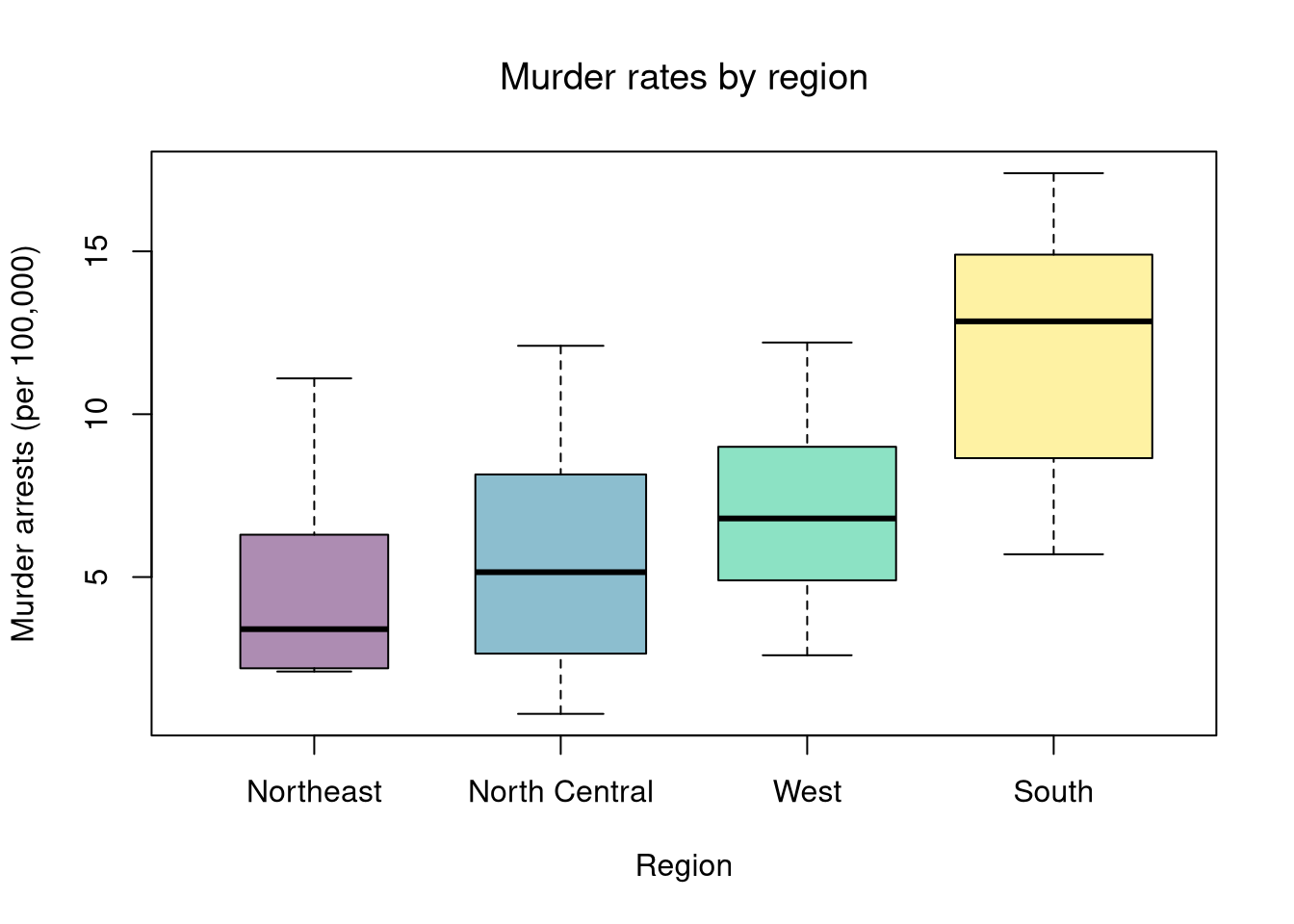
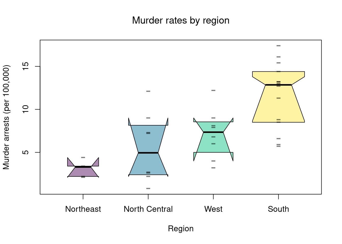
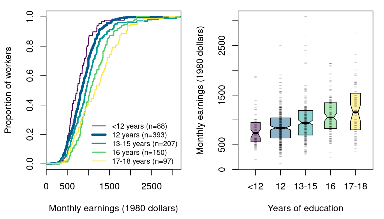
Comparing Two Groups split a cardinal outcome by a two-level factor and tested whether the two groups differed. This chapter extends that idea to \(G\) groups: how to describe several groups at once, how to compare their medians with bootstrap intervals, and then three ways to test whether they differ, one built on means, one built on ranks, and one built on category proportions.
Describing Groups
The census regions are an unordered factor with \(G=4\) levels. The built-in state.region vector lists them in the same state order as the rows of USArrests, so it can be paired directly with the murder rates. USArrests covers all \(50\) states, so it is the whole population of states rather than a sample from it. To make the bootstrap intervals below meaningful, pretend we observed only a random sample of \(35\) states, as we did with workers in Sampling.
Code
# Draw one random sample of 35 of the 50 states, and use only it from here on
set.seed(111)
state_id <- sample(nrow(USArrests), 35)

# Outcome: murder arrests per 100K, one value per sampled state
y_hat <- USArrests[state_id, 'Murder']
# Group: the four-level region factor, for the same sampled states.
# Its levels are the values the categorical variable can take.
region <- state.region[state_id]
levels(region)
## [1] "Northeast"     "South"         "North Central" "West"
table(region)
## region
##     Northeast         South North Central          West
##             5            14             8             8
Group Summaries
A factor with \(G\) levels splits a cardinal variable into \(G\) conditional distributions, one per group. The group summaries from Bivariate Distributions apply directly. The ECDF shows every observation, and drawing one per group on the same axes compares the whole distributions at once: a curve further to the right has higher values at every quantile. The regions are ordered by median murder rate from lowest to highest, so South is last in the legend, and each line’s thickness scales with its group size.
Code
# Order regions by their median murder rate, lowest to highest
region_order <- names(sort(tapply(y_hat, region, median)))
region <- factor(region, levels=region_order)

# One ECDF per region, on the same axes
line_cols <- hcl.colors(4)
n_g <- table(region)
lwd_g <- 1.5 + 2.5 * (n_g - min(n_g)) / (max(n_g) - min(n_g))

par(mar=c(4, 4, 4.5, 1))
plot(NULL, xlim=range(y_hat), ylim=c(0, 1),
    xlab='Murder arrests (per 100,000)', ylab='Proportion of states', main=NA)
for (g in seq_along(levels(region))) {
    F_g_hat <- ecdf(y_hat[region == levels(region)[g]])
    plot(F_g_hat, add=TRUE, col=line_cols[g], lwd=lwd_g[g],
        verticals=TRUE, do.points=FALSE, col.01line=NA)
}
legend('topleft', inset=c(0, -.2), xpd=TRUE, ncol=2, bty='n',
    legend=paste0(levels(region), ' (n=', n_g, ')'), col=line_cols, lty=1, lwd=lwd_g)
The South’s curve sits to the right of the others over its whole range, so its higher values are not driven by a few states.
A table of group sizes and centers puts numbers on the figure. The conditional mean \(\hat{m}_{Y}(g)\) is the average of \(\hat{y}_{i}\) among the \(n_g\) observations in group \(g\), and aggregate() computes it for every group at once.
Code
# Group size, mean, and median of the murder rate by region
summary_fun <- function(y_hat) {
    out <- c(n=length(y_hat), mean=mean(y_hat), median=median(y_hat))
    return(out)
}
aggregate(y_hat ~ region, FUN=summary_fun)
##          region  y_hat.n y_hat.mean y_hat.median
## 1     Northeast  5.00000    3.08000      3.30000
## 2 North Central  8.00000    5.48750      4.95000
## 3          West  8.00000    7.15000      7.35000
## 4         South 14.00000   11.58571     12.85000
The South has the highest center and the Northeast the lowest. Whether such differences are larger than chance alone would produce is the question the rest of this chapter takes up.
Equal Means (ANOVA)
In Comparing Groups, we tested whether two groups had the same mean. We now extend this to \(G\) groups. The Analysis of Variance (ANOVA) approach asks: are the observed differences in group means larger than we would expect from random variation alone?
Decomposition
If group means differ, some of the spread in \(\hat{y}\) must come from differences between groups rather than within them. We can split each piece out.
Label each observation \(\hat{y}_{ig}\) for individual \(i\) in group \(g\), where group \(g=1,\dots,G\) has \(n_g\) observations with group mean \(\hat{m}_{Y}(g)\), and the grand mean across all \(n=\sum_g n_g\) observations is \(\hat{m}_{Y}\). The ANOVA decomposition splits the total sum of squares into between-group and within-group pieces: \[\begin{aligned}
\underbrace{\sum_{g=1}^{G}\sum_{i=1}^{n_g}(\hat{y}_{ig}-\hat{m}_{Y})^2}_{\hat{\text{TSS}}}
&=
\underbrace{\sum_{g=1}^{G} n_g (\hat{m}_{Y}(g)-\hat{m}_{Y})^2}_{\hat{\text{BSS}}}
\;+\;
\underbrace{\sum_{g=1}^{G}\sum_{i=1}^{n_g}(\hat{y}_{ig}-\hat{m}_{Y}(g))^2}_{\hat{\text{WSS}}},
\end{aligned}\] where \(\hat{\text{BSS}}\) measures variation in group means around the grand mean and \(\hat{\text{WSS}}\) measures variation of observations around their own group mean.
The decomposition is useful as the foundation for any test of “do group means differ?”: if they do not, \(\hat{\text{BSS}}\) should be small relative to \(\hat{\text{WSS}}\). The equality holds exactly because the cross-term \(\sum_{g,i}(\hat{y}_{ig}-\hat{m}_{Y}(g))(\hat{m}_{Y}(g)-\hat{m}_{Y})\) vanishes, since the within-group deviations sum to zero around their own group mean.
In R, aov() fits the ANOVA model and summary() returns the standard ANOVA table. The ANOVA table reports \(\hat{\text{BSS}}\) (“Sum Sq” for region), \(\hat{\text{WSS}}\) (“Sum Sq” for Residuals).
Code
# Fit ANOVA
fit_aov <- aov(y_hat ~ region)
summary(fit_aov)
##             Df Sum Sq Mean Sq F value   Pr(>F)
## region       3  357.3  119.09   10.07 8.64e-05 ***
## Residuals   31  366.5   11.82
## ---
## Signif. codes:  0 '***' 0.001 '**' 0.01 '*' 0.05 '.' 0.1 ' ' 1
For example, suppose we have \(G=3\) groups with the following data:
Group means: \(\hat{m}_{Y}(A) = 5\), \(\hat{m}_{Y}(B) = 8\), \(\hat{m}_{Y}(C) = 6\). Grand mean: \(\hat{m}_Y = (5+8+6)/3 = 19/3 \approx 6.33\). Each group has \(n_g = 3\).
Between-group sum of squares: \[\begin{aligned}
\hat{\text{BSS}} &= 3(5-19/3)^2 + 3(8-19/3)^2 + 3(6-19/3)^2 \\
&= 3(16/9) + 3(25/9) + 3(1/9) = 48/9 + 75/9 + 3/9 = 14
\end{aligned}\] Within-group sum of squares: \[\begin{aligned}
\hat{\text{WSS}} &= [(4-5)^2+(5-5)^2+(6-5)^2] + [(8-8)^2+(7-8)^2+(9-8)^2] \\
& + [(5-6)^2+(6-6)^2+(7-6)^2] = 2+2+2 = 6
\end{aligned}\]
Code
# Data
y0_hat <- c(4, 5, 6, 8, 7, 9, 5, 6, 7)
g0 <- factor(c('A', 'A', 'A', 'B', 'B', 'B', 'C', 'C', 'C'))

# Verify by hand
m0_hat <- mean(y0_hat)
m0_g_hat <- aggregate(y0_hat, list(g0), mean)$x
n0_g <- aggregate(y0_hat, list(g0), length)$x

BSS <- sum(n0_g * (m0_g_hat - m0_hat)^2)
WSS <- sum(aggregate(y0_hat, list(g0), function(y_hat) sum((y_hat - mean(y_hat))^2))$x)
cbind(BSS, WSS)
##      BSS WSS
## [1,]  14   6
The F-statistic
We have the decomposition; now we need a single number that tells us when the between-group piece is “large” relative to the within-group piece.
The ANOVA \(F\)-statistic is the ratio of average between-group variation to average within-group variation: \[\hat{F} = \frac{\hat{\text{BSS}}/(G-1)}{\hat{\text{WSS}}/(n-G)}.\] Writing \(Y_{ig}\) for the random outcome of individual \(i\) in group \(g\), the null is \(H_0: \mathbb{E}[Y_{i1}]=\mathbb{E}[Y_{i2}]=\dots=\mathbb{E}[Y_{iG}]\).
The ANOVA F-statistic is useful as the global “do any means differ?” test: one number and one \(p\)-value, regardless of how many groups you have. A large \(\hat{F}\) means the group means are more spread out than individual-level noise would predict.
Code
F_fun <- function(y_hat,g){
    m_y_hat <- mean(y_hat)
    m_g_hat <- aggregate(y_hat, list(g), mean)$x
    n_g <- aggregate(y_hat, list(g), length)$x

    BSS <- sum(n_g * (m_g_hat - m_y_hat)^2)
    WSS <- sum(aggregate(y_hat, list(g), function(y_hat) sum((y_hat - mean(y_hat))^2))$x)

    n <- length(y_hat)
    G <- nlevels(g)
    F_obs <- (BSS/(G-1)) / (WSS/(n-G))
    return(F_obs)
}
F_obs <- F_fun(y_hat=y_hat, g=region)
F_obs
## [1] 10.0743
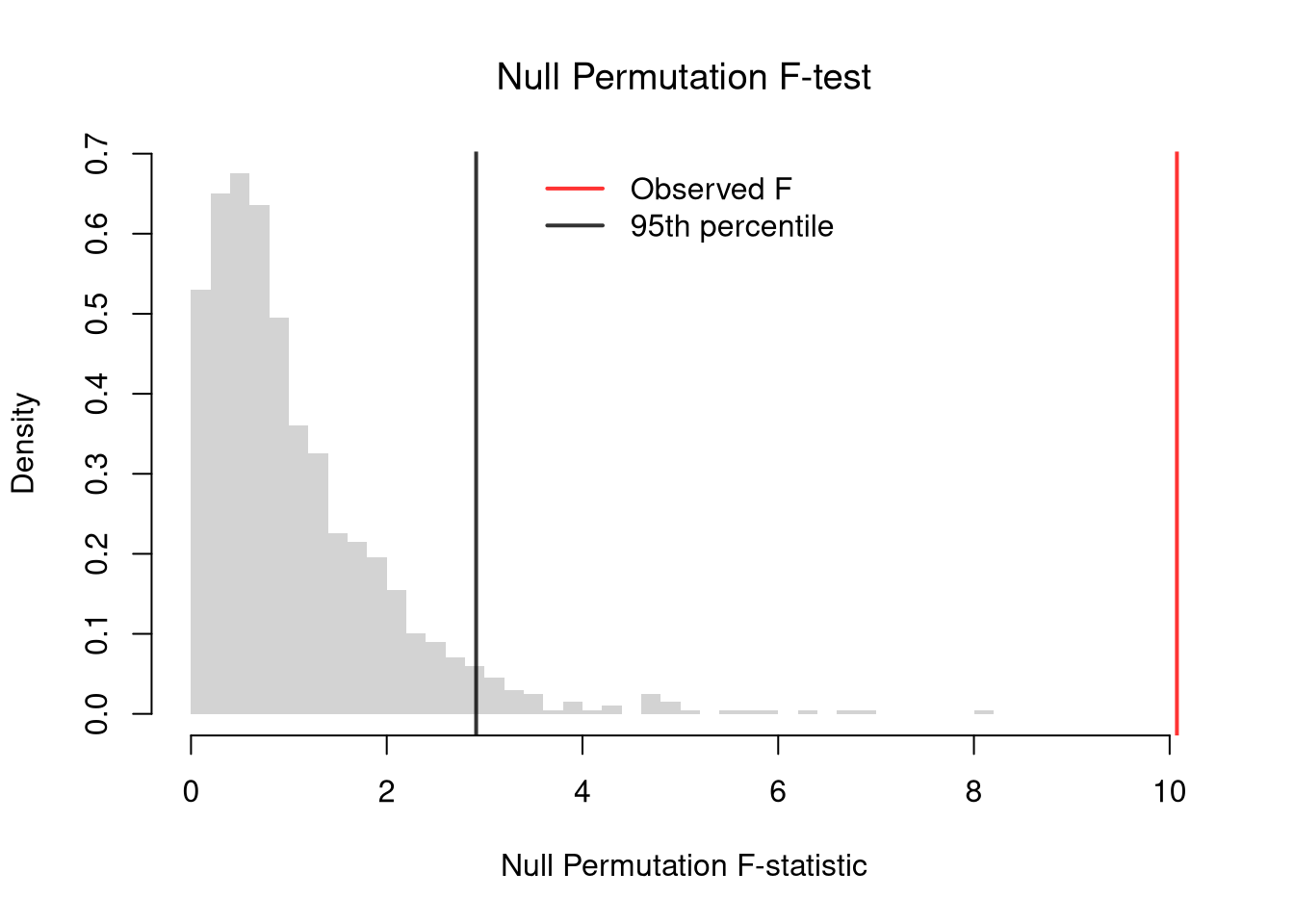
To compute a \(p\)-value, we use a permutation test: shuffle the region labels, which keeps each region’s number of states fixed, and recompute \(\hat{F}\) each time. Only large values of \(\hat{F}\) count against the null. As with KS and CVM in Comparing Two Groups, we reject at the \(5\%\) level when \(\hat{F}\) exceeds the \(95\)th percentile of the permutation distribution.
Code
# Null distribution: shuffle region labels to break the Y--group pairing
F_perm <- vector(length=999)
for( b in seq_along(F_perm)){
    g_perm <- sample(region, replace=FALSE)
    F_perm[b] <- F_fun(y_hat=y_hat, g=g_perm)
}

# Permutation p-value
p_perm <- mean(F_perm >= F_obs)
p_perm
## [1] 0

# One-sided critical value: 95th percentile of the permutation distribution
F_crit <- quantile(F_perm, probs=.95)

hist(F_perm, breaks = 40,
    border = NA,
    freq = FALSE, main = NA, xlab = 'Null Permutation F-statistic',
    xlim = range(c(0, F_perm, F_obs)))
title('Null Permutation F-test', font.main = 1)
abline(v = F_crit, col = rgb(0, 0, 0, .8), lwd = 2)
abline(v = F_obs, col = rgb(1, 0, 0, .8), lwd = 2)
legend('top', legend = c('Observed F', '95th percentile'),
    col = c(rgb(1, 0, 0, .8), rgb(0, 0, 0, .8)), lwd = 2, bty='n')
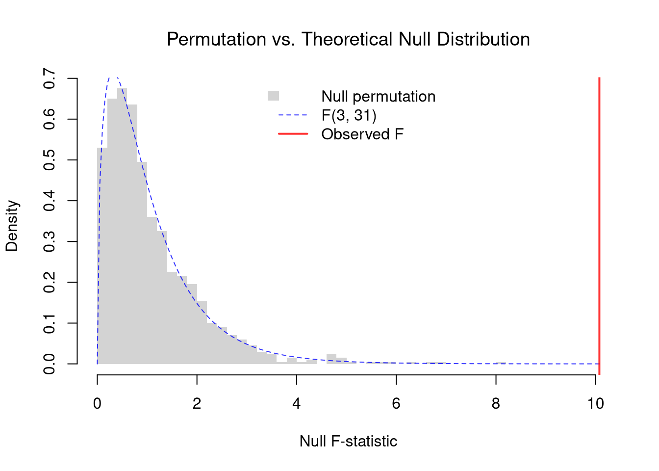
Pairing the observed murder rates y_hat with a shuffled region vector breaks the link between outcome and group: under the null, group labels are exchangeable, so this approximates the distribution of \(\hat{F}\) when no group effect exists.
Under the null and additional parametric assumptions, \(\hat{F}\) follows an \(F_{G-1,\;n-G}\) distribution. The parametric \(F_{G-1,\;n-G}\) null distribution requires three assumptions: independent observations, normal errors within each group, and equal variances across groups (homoscedasticity). R reports \(p\)-values from this theoretical distribution by default.
The figure below draws the theoretical \(F_{G-1,\;n-G}\) density over the permutation distribution from above.
Code
# Degrees of freedom for the regional data
n <- length(y_hat)
G <- nlevels(region)
p_param <- 1 - pf(F_obs, G-1, n-G)

# Compare parametric and permutation p-values
cbind(F_obs, p_param, p_perm)
##        F_obs      p_param p_perm
## [1,] 10.0743 8.639652e-05      0

# Overlay: permutation histogram vs. theoretical F density
hist(F_perm, breaks = 40,
    border = NA,
    freq = FALSE, main = NA, xlab = 'Null F-statistic',
    xlim = range(c(0, F_perm, F_obs)))
title('Permutation vs. Theoretical Null Distribution', font.main = 1)
F_grid <- seq(0, max(c(F_perm, F_obs)), length = 200)
lines(F_grid, df(F_grid, G-1, n-G), col = rgb(0, 0, 1, .8), lwd = 1, lty = 2)
abline(v = F_obs, col = rgb(1, 0, 0, .8), lwd = 2)
legend('top', legend = c('Null permutation', paste0('F(', G-1, ', ', n-G, ')'), 'Observed F'),
    fill = c(grey(.83), NA, NA), border = NA, # grey(.83) matches the default histogram fill
    lwd = c(NA, 1, 2), lty = c(NA, 2, 1), col = c(NA, rgb(0, 0, 1, .8), rgb(1, 0, 0, .8)), bty = 'n')
If these assumptions are doubtful, the Kruskal-Wallis test below is a safer alternative. As a quick check, compare side-by-side boxplots: if the spread differs across groups or the distributions show strong skewness or kurtosis, be cautious with the parametric test.
For the three-group example above, \(\hat{F}=(14/2)/(6/6)=7\). With \(G-1=2\) and \(n-G=6\) degrees of freedom, we compare it to an \(F_{2,6}\) distribution: \(p = 1 - F_{2,6}(7) \approx 0.027\).
Code
# Data (the three-group example from the decomposition above)
y0_hat <- c(4, 5, 6, 8, 7, 9, 5, 6, 7)
g0 <- factor(c('A', 'A', 'A', 'B', 'B', 'B', 'C', 'C', 'C'))

# Computation
summary(aov(y0_hat ~ g0))
##             Df Sum Sq Mean Sq F value Pr(>F)
## g0           2     14       7       7  0.027 *
## Residuals    6      6       1
## ---
## Signif. codes:  0 '***' 0.001 '**' 0.01 '*' 0.05 '.' 0.1 ' ' 1

# Verify by hand
n0 <- length(y0_hat)
G0 <- nlevels(g0)
m0_hat <- mean(y0_hat)
m0_g_hat <- aggregate(y0_hat, list(g0), mean)$x
n0_g <- aggregate(y0_hat, list(g0), length)$x
BSS <- sum(n0_g * (m0_g_hat - m0_hat)^2)
WSS <- sum(aggregate(y0_hat, list(g0), function(y_hat) sum((y_hat - mean(y_hat))^2))$x)
Fstat <- (BSS/(G0-1)) / (WSS/(n0-G0))
pval  <- 1 - pf(Fstat, G0-1, n0-G0)
cbind(BSS, WSS, Fstat, pval)
##      BSS WSS Fstat  pval
## [1,]  14   6     7 0.027
Equal Distributions
ANOVA tests whether group means differ; sometimes the entire distributions differ in ways the mean would miss.
Kruskal-Wallis Test
When data are skewed, heavy-tailed, or only ordinal, a test built on means may overlook differences that show up in the rank order.
The Kruskal-Wallis test is a nonparametric test for equal distributions across \(G\) groups, testing \(H_0: F_1 = F_2 = \dots = F_G\) against \(H_A:\) at least one \(F_g\) differs (where \(F_g\) is the continuous distribution of group \(g=1,...G\)). It uses the average ranks within each group rather than the raw observations, so it only requires the data to be ordinal. With two groups it reduces to the Mann-Whitney U (equivalently Wilcoxon rank-sum) test.
The Kruskal-Wallis test is useful when the equal-variance normal-error assumption is implausible, as with income, response times, or other heavy-tailed outcomes. Rank-based tests need only the orderings of the data. A significant result tells us that some distribution differs, but not which one; the global rejection has to be followed up with pairwise tests.
To conduct the test, first denote individuals \(i=1,...n\) with overall ranks \(\hat{r}_1,....\hat{r}_{n}\). Each individual belongs to group \(g=1,...G\), and each group \(g\) has \(n_{g}\) individuals with average rank \(\bar{r}_{g} = \sum_{i} \hat{r}_{i} /n_{g}\). The Kruskal Wallis statistic is \[\begin{aligned}
\hat{\text{KW}} &= (n-1) \frac{\sum_{g=1}^{G} n_{g}( \bar{r}_{g} - \bar{r} )^2 }{\sum_{i=1}^{n} ( \hat{r}_{i} - \bar{r} )^2},
\end{aligned}\] where \(\bar{r} = \frac{n+1}{2}\) is the grand mean rank.
In the special case with only two groups, the Kruskal Wallis test reduces to the Mann–Whitney U test (also known as the Wilcoxon rank-sum test). In this case, we can write the hypotheses in terms of individual outcomes in each group, \(Y_i\) in one group \(Y_j\) in the other; \(H_0: \text{Prob}(Y_i > Y_j)=\text{Prob}(Y_j > Y_i)\) versus \(H_A: \text{Prob}(Y_i > Y_j) \neq \text{Prob}(Y_j > Y_i)\). The corresponding test statistic is \[\begin{aligned}
\hat{U} &= \min(\hat{U}_1, \hat{U}_2) \\
\hat{U}_g &= \sum_{i~\text{in}~g}\sum_{j~\text{in}~-g}
\Bigl[\mathbf 1( \hat{y}_{i} > \hat{y}_{j}) + \tfrac12\mathbf 1(\hat{y}_{i} = \hat{y}_{j})\Bigr].
\end{aligned}\]
Interpretation template:
- If the Kruskal-Wallis p-value is large, keep the global null and stop.
- If the p-value is small, report that at least one group differs.
- Report both statistical and practical importance (distribution plots + effect size summaries), not only p-values.
Code
kw <- kruskal.test(y_hat ~ region)
kw
##
##  Kruskal-Wallis rank sum test
##
## data:  y_hat by region
## Kruskal-Wallis chi-squared = 16.394, df = 3, p-value = 0.0009415
A significant Kruskal-Wallis result tells us that some group differs, not which. To answer which, use a post-hoc pairwise test together with a multiple-comparisons correction. Here, pairwise.wilcox.test() runs a Mann-Whitney test on each pair of regions, and the Holm correction adjusts the \(p\)-values for the number of pairs tested.
Code
pairwise.wilcox.test(y_hat, region, p.adjust.method='holm')
##
##  Pairwise comparisons using Wilcoxon rank sum exact test
##
## data:  y_hat and region
##
##               Northeast North Central West
## North Central 0.582     -             -
## West          0.075     0.582         -
## South         0.001     0.031         0.075
##
## P value adjustment method: holm
Looking back at the boxplot in Equal Medians, which region stands out?
Worked example: \(G=3\) groups with values \(A=\{1,2,3\}\), \(B=\{4,5,6\}\), \(C=\{7,8,9\}\).
Pooling and ranking gives the ranks \(1,\ldots,9\) in order. Group rank averages: \(\bar{r}_A=2\), \(\bar{r}_B=5\), \(\bar{r}_C=8\). Grand mean rank: \(\bar{r}=(n+1)/2=5\). Plug into \(\hat{\text{KW}}\) with \(n=9\), \(n_g=3\): \[
\hat{\text{KW}} = (n-1) \cdot \frac{3(2-5)^2 + 3(5-5)^2 + 3(8-5)^2}{\sum_{i=1}^{9}(\hat{r}_i - 5)^2}
= 8 \cdot \frac{27 + 0 + 27}{60} = 7.2.
\]
Code
y0_hat <- c(1,2,3, 4,5,6, 7,8,9)
g0 <- factor(rep(c('A','B','C'), each=3))
kruskal.test(y0_hat ~ g0)
##
##  Kruskal-Wallis rank sum test
##
## data:  y0_hat by g0
## Kruskal-Wallis chi-squared = 7.2, df = 2, p-value = 0.02732
For the two-group case, the Mann-Whitney statistic counts pairwise wins. Compare \(A=\{1,3,5\}\) to \(B=\{2,4,6\}\): out of \(3\times 3 = 9\) pairs, \(A\) wins three (\((3,2), (5,2), (5,4)\)), so \(\hat{U}_A=3\), \(\hat{U}_B=6\), giving \(\hat{U}=\min(3,6)=3\).
Code
a0_hat <- c(1,3,5); b0_hat <- c(2,4,6)
wilcox.test(a0_hat, b0_hat)
##
##  Wilcoxon rank sum exact test
##
## data:  a0_hat and b0_hat
## W = 3, p-value = 0.7
## alternative hypothesis: true location shift is not equal to 0
Categorical ANOVA
When the outcome is a factor, we can still ask whether the groups spread their observations across the categories in the same proportions. Let \(\hat{p}(y)\) be the proportion of all \(n\) observations in category \(y\), and \(\hat{p}(y \mid g)\) the proportion of the \(n_g\) observations in group \(g\). The categorical ANOVA measures variation with one minus the Herfindahl index, and splits it into between-group and within-group pieces: \[\begin{aligned}
\underbrace{\frac{n}{2}\left(1-\hat{H}\right)}_{\hat{\text{TSS}}}
&=
\underbrace{\frac{1}{2}\sum_{g=1}^{G} n_g \sum_{y}\left(\hat{p}(y \mid g)-\hat{p}(y)\right)^2}_{\hat{\text{BSS}}}
\;+\;
\underbrace{\sum_{g=1}^{G} \frac{n_g}{2}\left(1-\hat{H}(g)\right)}_{\hat{\text{WSS}}},
\end{aligned}\] where \(\hat{H}=\sum_{y}\hat{p}(y)^2\) is the Herfindahl index of the pooled data and \(\hat{H}(g)=\sum_{y}\hat{p}(y \mid g)^2\) is the Herfindahl index within group \(g\).
The categorical ANOVA is useful when the outcome is an unordered factor, such as occupation, brand, or vote choice, where there are no means to compare and no ranks to sort. Recall that \(1-\hat{H}\) is zero when every observation falls in one category and grows as the categories become equally common, so it plays the role of the variance. The pieces are also ordinary ANOVA sums of squares. Make one 0/1 indicator for each category and compute its \(\hat{\text{TSS}}\), \(\hat{\text{BSS}}\), and \(\hat{\text{WSS}}\) as in the decomposition above. Adding each piece up across the categories and halving it gives the three pieces here. With a binary outcome, the two indicators have the same sums of squares, so the categorical ANOVA is exactly the ANOVA of a single 0/1 variable. The share \(\hat{\text{BSS}}/\hat{\text{TSS}}\) reports the fraction of the variation in \(\hat{y}\) that lies between groups.
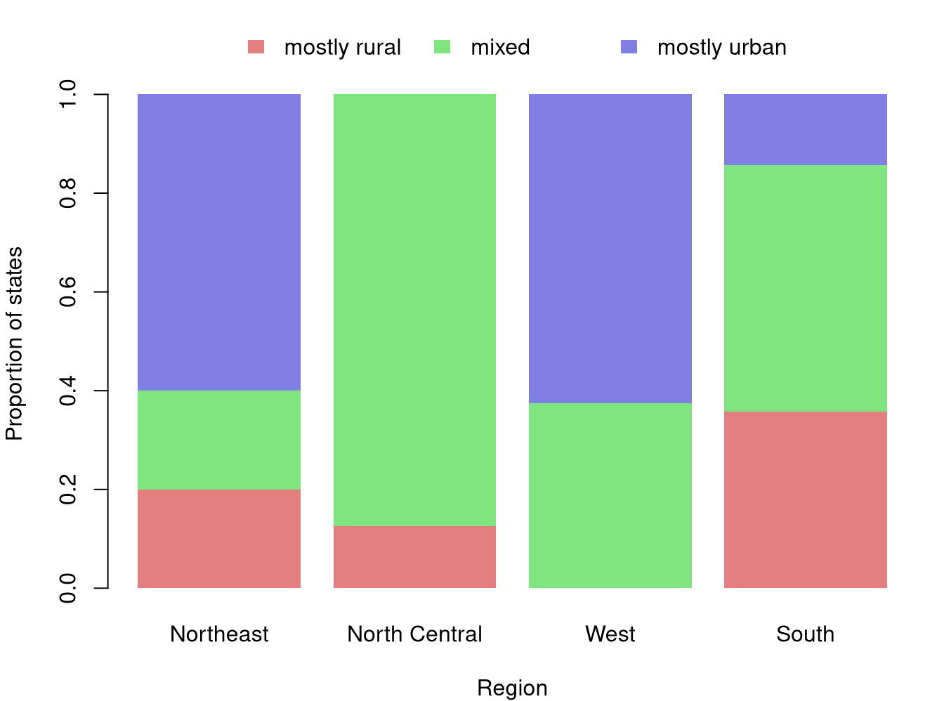
For example, the urban population bands from Ordered Factors sort each region’s states into mostly rural, mixed, and mostly urban. The bands are ordered, but the categorical ANOVA ignores that order, so it treats them as it would any unordered factor.
Code
# Outcome: urban population in three bands, an ordered factor, for the sampled states
urban_band <- cut(USArrests[state_id, 'UrbanPop'], breaks=c(0, 50, 75, 100),
    labels=c('mostly rural', 'mixed', 'mostly urban'), ordered_result=TRUE)
tab <- table(region, urban_band)
tab
##                urban_band
## region          mostly rural mixed mostly urban
##   Northeast                1     1            3
##   North Central            1     7            0
##   West                     0     3            5
##   South                    5     7            2

# Proportions within each region: each bar sums to 1
p_band_region <- prop.table(tab, 1)
cols <- c(rgb(.8, 0, 0, .5), rgb(0, .8, 0, .5), rgb(0, 0, .8, .5))
par(mar=c(4, 4, 3.5, 1))
barplot(t(p_band_region), col=cols, border=NA,
    xlab='Region', ylab='Proportion of states', main=NA)
legend('top', inset=c(0, -.15), xpd=TRUE, ncol=3, bty='n',
    fill=cols, border=NA, legend=levels(urban_band))
The South and North Central lean rural, while the Northeast and West lean urban. The function below computes the three pieces and the between-group share.
Code
# Categorical ANOVA: variation is measured by one minus the Herfindahl index
cat_anova <- function(y_hat, g) {
    # Total variation, from the pooled proportions
    n <- length(y_hat)
    p_hat <- table(y_hat) / n
    TSS <- n / 2 * (1 - sum(p_hat^2))
    # Within-group variation, from each group's own proportions
    WSS_g <- tapply(y_hat, g, function(y_g) {
        p_g_hat <- table(y_g) / length(y_g)
        return(length(y_g) / 2 * (1 - sum(p_g_hat^2)))
    })
    WSS <- sum(WSS_g)
    # Between-group variation, from the decomposition
    BSS <- TSS - WSS
    return(c(BSS=BSS, WSS=WSS, TSS=TSS, share=BSS / TSS))
}
cat_anova(urban_band, region)
##        BSS        WSS        TSS      share
##  2.3785714  8.3642857 10.7428571  0.2214096
About \(22\%\) of the variation in urban bands lies between regions.
Suppose we record how \(n=8\) workers commute, \(n_g=4\) from each of two neighborhoods. Neighborhood \(A\) has car, car, car, bus, and neighborhood \(B\) has car, bus, bike, bike.
Pooled, the proportions are \(\hat{p}(\text{car})=4/8\), \(\hat{p}(\text{bus})=2/8\), and \(\hat{p}(\text{bike})=2/8\), so \(\hat{H}=1/4+1/16+1/16=3/8\) and \(\hat{\text{TSS}}=\frac{8}{2}(1-3/8)=5/2\). Within \(A\), \(\hat{H}(A)=(3/4)^2+(1/4)^2=5/8\), and within \(B\), \(\hat{H}(B)=(1/4)^2+(1/4)^2+(2/4)^2=3/8\). So \(\hat{\text{WSS}}=\frac{4}{2}(1-5/8)+\frac{4}{2}(1-3/8)=3/4+5/4=2\). For \(\hat{\text{BSS}}\), each neighborhood’s proportions differ from the pooled ones by \(1/4\) in two categories and by \(0\) in the third, so \(\hat{\text{BSS}}=\frac{1}{2}[4(1/16+0+1/16)+4(1/16+0+1/16)]=1/2\). The pieces add up, \(5/2=1/2+2\), and the between-group share is \(\hat{\text{BSS}}/\hat{\text{TSS}}=1/5\).
Code
# Commute mode of 8 workers, 4 from each neighborhood
y0_hat <- factor(c('car', 'car', 'car', 'bus', 'car', 'bus', 'bike', 'bike'))
g0 <- factor(c('A', 'A', 'A', 'A', 'B', 'B', 'B', 'B'))
table(g0, y0_hat)
##    y0_hat
## g0  bike bus car
##   A    0   1   3
##   B    2   1   1
cat_anova(y0_hat, g0)
##   BSS   WSS   TSS share
##   0.5   2.0   2.5   0.2
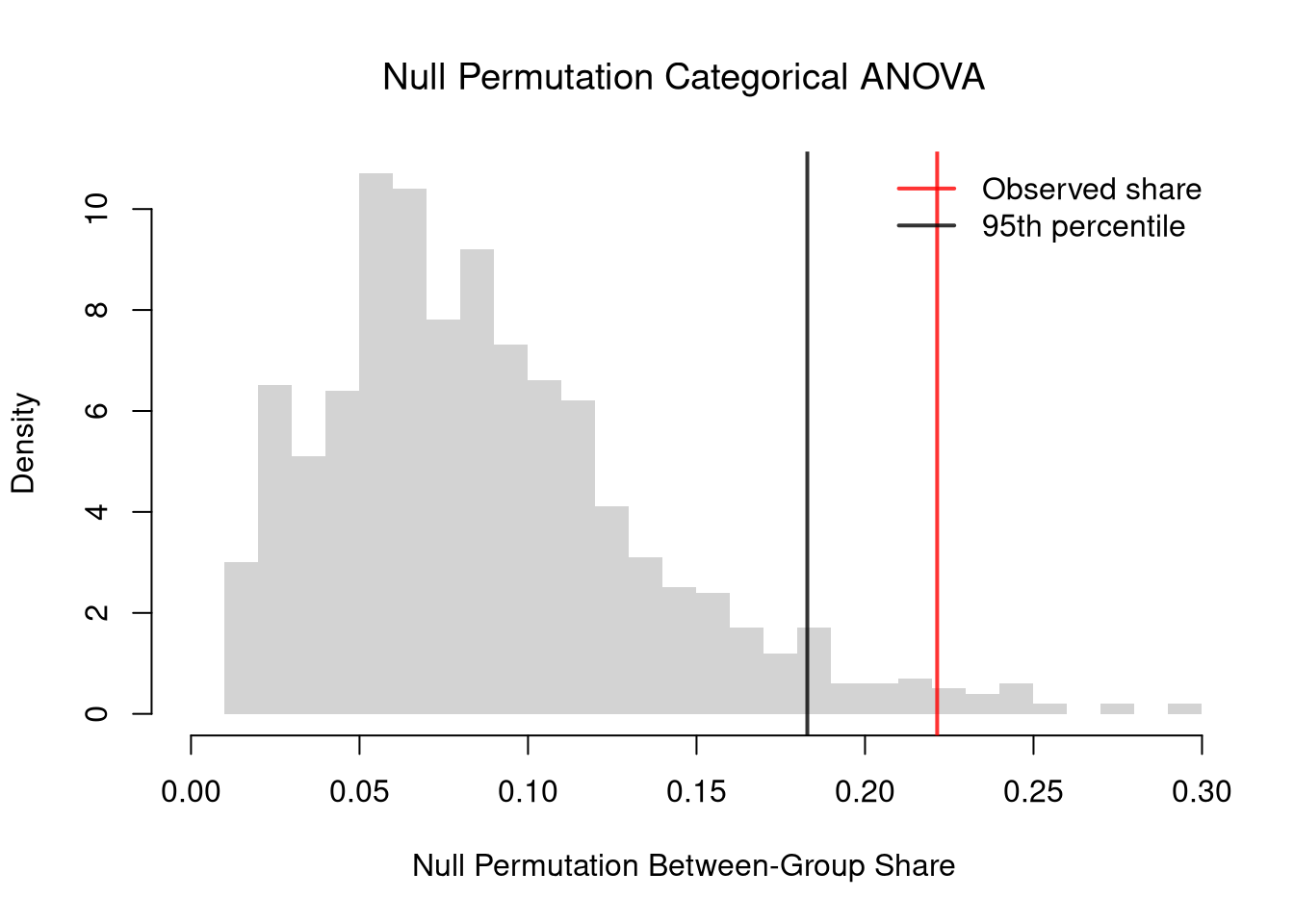
As with the ANOVA \(F\)-statistic, we get a \(p\)-value by shuffling the region labels and recomputing the share each time.
Code
# Observed between-group share
share_obs <- cat_anova(urban_band, region)[['share']]

# Null distribution: shuffle region labels to break the outcome--group pairing
share_perm <- rep(NA, 999)
for (b in seq_along(share_perm)) {
    g_perm <- sample(region, replace=FALSE)
    share_perm[b] <- cat_anova(urban_band, g_perm)[['share']]
}

# Permutation p-value
p_perm <- mean(share_perm >= share_obs)
p_perm
## [1] 0.02002002

# One-sided critical value: 95th percentile of the permutation distribution
share_crit <- quantile(share_perm, probs=.95)

hist(share_perm, breaks=40,
    border=NA,
    freq=FALSE, main=NA, xlab='Null Permutation Between-Group Share',
    xlim=range(c(0, share_perm, share_obs)))
title('Null Permutation Categorical ANOVA', font.main=1)
abline(v=share_crit, col=rgb(0, 0, 0, .8), lwd=2)
abline(v=share_obs, col=rgb(1, 0, 0, .8), lwd=2)
legend('topright', legend=c('Observed share', '95th percentile'),
    col=c(rgb(1, 0, 0, .8), rgb(0, 0, 0, .8)), lwd=2, bty='n')
Because the bands are ordered, the Kruskal-Wallis test also applies.
Code
# Kruskal-Wallis ranks the bands, so it uses their order
kruskal.test(urban_band ~ region)
##
##  Kruskal-Wallis rank sum test
##
## data:  urban_band by region
## Kruskal-Wallis chi-squared = 9.284, df = 3, p-value = 0.02574
Here the categorical ANOVA gives the smaller \(p\)-value. The regions differ partly along one direction, from rural to urban, and ranks concentrate on that direction. The categorical ANOVA spreads its attention over every way the proportions could differ, so a rank test is usually more powerful when the categories are ordered. The categorical ANOVA can still detect differences that ranks miss, such as one group concentrated in the middle band and another split between the two extremes. In this sample, \(7\) of North Central’s \(8\) states are in the middle band. That pattern contributes more to the categorical ANOVA than any other region does, but the least to the Kruskal-Wallis statistic.
Make a binary outcome that marks the mostly urban states. Check that the categorical ANOVA of this outcome gives the same \(\hat{\text{BSS}}\) and \(\hat{\text{WSS}}\) as the ordinary ANOVA of the 0/1 variable.
Code
# 1 for mostly urban states, 0 otherwise
d_hat <- as.numeric(urban_band == 'mostly urban')
cat_anova(factor(d_hat), region)
##      BSS      WSS      TSS    share
## 2.353571 4.789286 7.142857 0.329500
summary(aov(d_hat ~ region))
##             Df Sum Sq Mean Sq F value  Pr(>F)
## region       3  2.354  0.7845   5.078 0.00563 **
## Residuals   31  4.789  0.1545
## ---
## Signif. codes:  0 '***' 0.001 '**' 0.01 '*' 0.05 '.' 0.1 ' ' 1
Exercises
Comment the script you wrote for this chapter, then restart R and check that it runs from a clean session, then check the script with AI as explained in Working with AI. Write three sentences from memory on the main statistical idea of this chapter, and ask the assistant what is wrong, vague, or missing. Finish with your own questions about whatever you found hardest.
Load Wages1 from the Ecdat package. Draw a boxplot of wage by sex, then add an ECDF of wage for each sex on the same axes. Compute the mean and median wage for each sex with aggregate(). Does one sex’s ECDF sit to the right of the other’s over the whole range, or do the curves cross?
An ANOVA \(F\)-test rejects the null that all group means are equal. Does this tell you which group is different, or only that at least one differs?
Using the USArrests dataset with state.region as the grouping variable, compute the between-group sum of squares (\(\hat{\text{BSS}}\)) and within-group sum of squares (\(\hat{\text{WSS}}\)) for Assault by hand (using aggregate()). Verify your \(\hat{F}\) statistic matches the output of summary(aov(Assault ~ state.region, data = ...)).
Recall
This chapter first described several groups with ECDFs and a table of group means, compared their medians with bootstrap notches on boxplots, and then tested whether the description reflected more than chance. ANOVA’s decomposition of variation between and within groups produced an \(F\)-statistic; the worked three-group example with \(A=\{4,5,6\}, B=\{8,7,9\}, C=\{5,6,7\}\) made the arithmetic concrete, giving \(\hat{\text{BSS}}=14\) and \(\hat{\text{WSS}}=6\) by hand, which aov(y0_hat ~ g0) reproduces exactly. The Kruskal-Wallis test replaced outcomes with ranks when the equal-variance normal-error assumptions were doubtful. The categorical ANOVA measured the variation of a factor outcome with one minus the Herfindahl index; for the commutes in two neighborhoods it gave \(\hat{\text{TSS}}=5/2\), \(\hat{\text{BSS}}=1/2\), and \(\hat{\text{WSS}}=2\) by hand.