Code
dat <- USArrests
dat$Region <- state.region
levels(dat$Region)
## [1] "Northeast" "South" "North Central" "West"So far, we have discussed cardinal data where the difference between units always means the same thing: e.g., \(4-3=2-1\). There are also factor variables
To analyze either factor, we often convert them into indicator variables or dummies; \(\hat{D}_{c}=\mathbf{1}( \text{Factor} = c)\). One common case is if you have observations of individuals over time periods, then you may have two factor variables. An unordered factor that indicates who an individual is; for example \(\hat{D}_{i}=\mathbf{1}( \text{Individual} = i)\), and an order factor that indicates the time period; for example \(\hat{D}_{t}=\mathbf{1}( \text{Time} \in [\text{month}~ t, \text{month}~ t+1) )\). There are many other cases you see factor variables, including spatial ID’s in purely cross sectional data.
Be careful not to handle categorical data as if they were cardinal. E.g., generate city data with Leipzig=1, Lausanne=2, LosAngeles=3, … and then include city as if it were a cardinal number (that’s a big no-no). The same applied to ordinal data; PopulationLeipzig=2, PopulationLausanne=3, PopulationLosAngeles=1.
In this chapter, we use state.region (Northeast, South, North Central, West) as an unordered factor to group the USArrests data by US Census region.
dat <- USArrests
dat$Region <- state.region
levels(dat$Region)
## [1] "Northeast" "South" "North Central" "West"With multiple groups, begin with a summary figure (such as a boxplot) and then run a global test of whether at least one group differs.
# Step 1: Visual summary
boxplot(Murder ~ Region, data = dat,
    col = hcl.colors(4, alpha = .45),
    ylab = 'Murder arrests (per 100k)', xlab = 'Region', main = NA)
title('Murder rates by region', font.main = 1)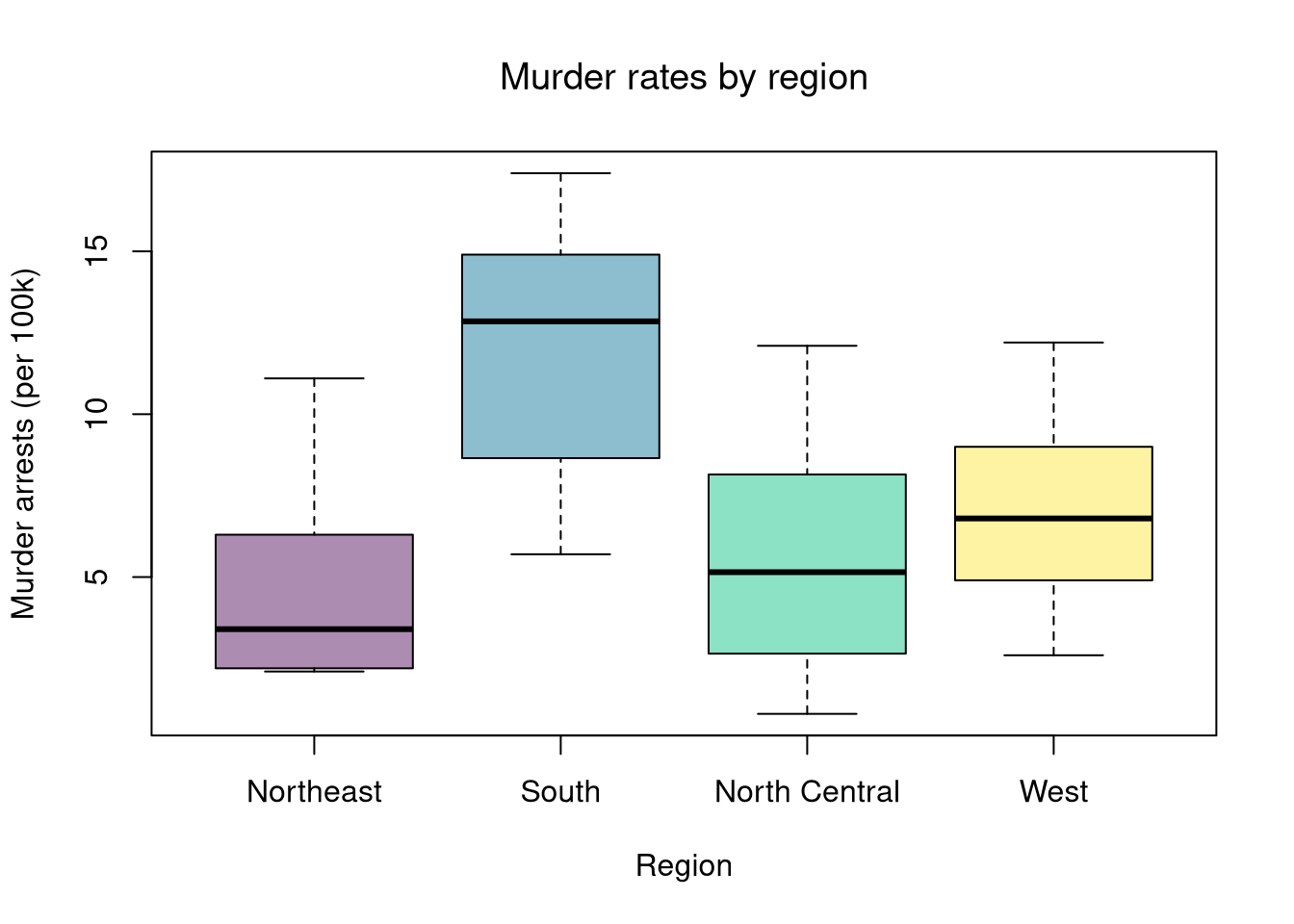
In Comparing Groups, we tested whether two groups had the same mean. We now extend this to \(G\) groups. The Analysis of Variance (ANOVA) approach asks: are the observed differences in group means larger than we would expect from random variation alone?
The key idea is to decompose total variation into between-group and within-group components. Label each observation \(\hat{Y}_{ig}\) for individual \(i\) in group \(g\). Each group \(g=1,\dots,G\) has \(n_g\) observations with group mean \(\hat{M}_{g}\), and the grand mean across all \(n=\sum_g n_g\) observations is \(\hat{M}_{Y}\). Then the total sum of squares decomposes as \[\begin{eqnarray} \underbrace{\sum_{g=1}^{G}\sum_{i=1}^{n_g}(\hat{Y}_{ig}-\hat{M}_{Y})^2}_{\hat{TSS}} &=& \underbrace{\sum_{g=1}^{G} n_g (\hat{M}_{g}-\hat{M}_{Y})^2}_{\hat{BSS}} \;+\; \underbrace{\sum_{g=1}^{G}\sum_{i=1}^{n_g}(\hat{Y}_{ig}-\hat{M}_{g})^2}_{\hat{WSS}}, \end{eqnarray}\] where \(\hat{BSS}\) is the between-group sum of squares (variation in group means around the grand mean) and \(\hat{WSS}\) is the within-group sum of squares (variation of observations around their own group mean).
If the group means are all equal, then \(\hat{BSS}\) should be small relative to \(\hat{WSS}\).
In R, aov() fits the ANOVA model and summary() returns the standard ANOVA table. The ANOVA table reports \(\hat{BSS}\) (“Sum Sq” for Region), \(\hat{WSS}\) (“Sum Sq” for Residuals).
# Fit ANOVA
fit_aov <- aov(Murder ~ Region, data = dat)
fit_aov
## Call:
##    aov(formula = Murder ~ Region, data = dat)
##
## Terms:
##                   Region Residuals
## Sum of Squares  391.2357  538.3171
## Deg. of Freedom        3        46
##
## Residual standard error: 3.420898
## Estimated effects may be unbalancedWe test \(H_0: \mu_1=\mu_2=\dots=\mu_G\) versus \(H_A:\) at least one \(\mu_g\) differs. The ANOVA F-statistic is \[\begin{eqnarray} \hat{F} &=& \frac{\hat{BSS}/(G-1)}{\hat{WSS}/(n-G)}. \end{eqnarray}\] The numerator is the average between-group variation (per degree of freedom), and the denominator is the average within-group variation. A large \(\hat{F}\) means group means are more spread out than individual-level noise would predict.
F_fun <- function(Y,g){
    M_Y <- mean(Y)
    M_g <- aggregate(Y, list(g), mean)$x
    n_g <- aggregate(Y, list(g), length)$x

    BSS <- sum(n_g * (M_g - M_Y)^2)
    WSS <- sum(aggregate(Y, list(g), function(y) sum((y - mean(y))^2))$x)

    n <- nrow(dat)
    G <- nlevels(g)
    F_obs <- (BSS/(G-1)) / (WSS/(n-G))
}
F_obs <- F_fun(Y=dat$Murder, g=dat$Region)
F_obs
## [1] 11.14389
To compute a \(p\)-value, we can use permutation or bootstrap methods to build a null distribution, just as in previous chapters.
# Pairs bootstrap: resample rows with replacement
B <- 5000
n <- nrow(dat)

F_nullboot <- vector(length=999)
for( b in seq_along(F_nullboot)){
    idx <- sample(n, replace = TRUE)
    g_boot <- dat[idx, 'Region']
    F_b <- F_fun(Y=dat$Murder, g=g_boot)
    F_nullboot[b] <- F_b
}

# Bootstrap p-value
p_boot <- mean(F_nullboot >= F_obs)
p_boot
## [1] 0

hist(F_nullboot, breaks = 40,
    col = grey(0.5, 0.5), border = NA,
    freq = F, main = NA, xlab = 'Null Bootstrap F-statistic',
    xlim = c(0,14))
title('Null Bootstrap F-test', font.main = 1)
abline(v = F_obs, col = rgb(1, 0, 0, .8), lwd = 2)
legend('topright', legend = 'Observed F',
    col = rgb(1, 0, 0, .8), lwd =0, bty='n')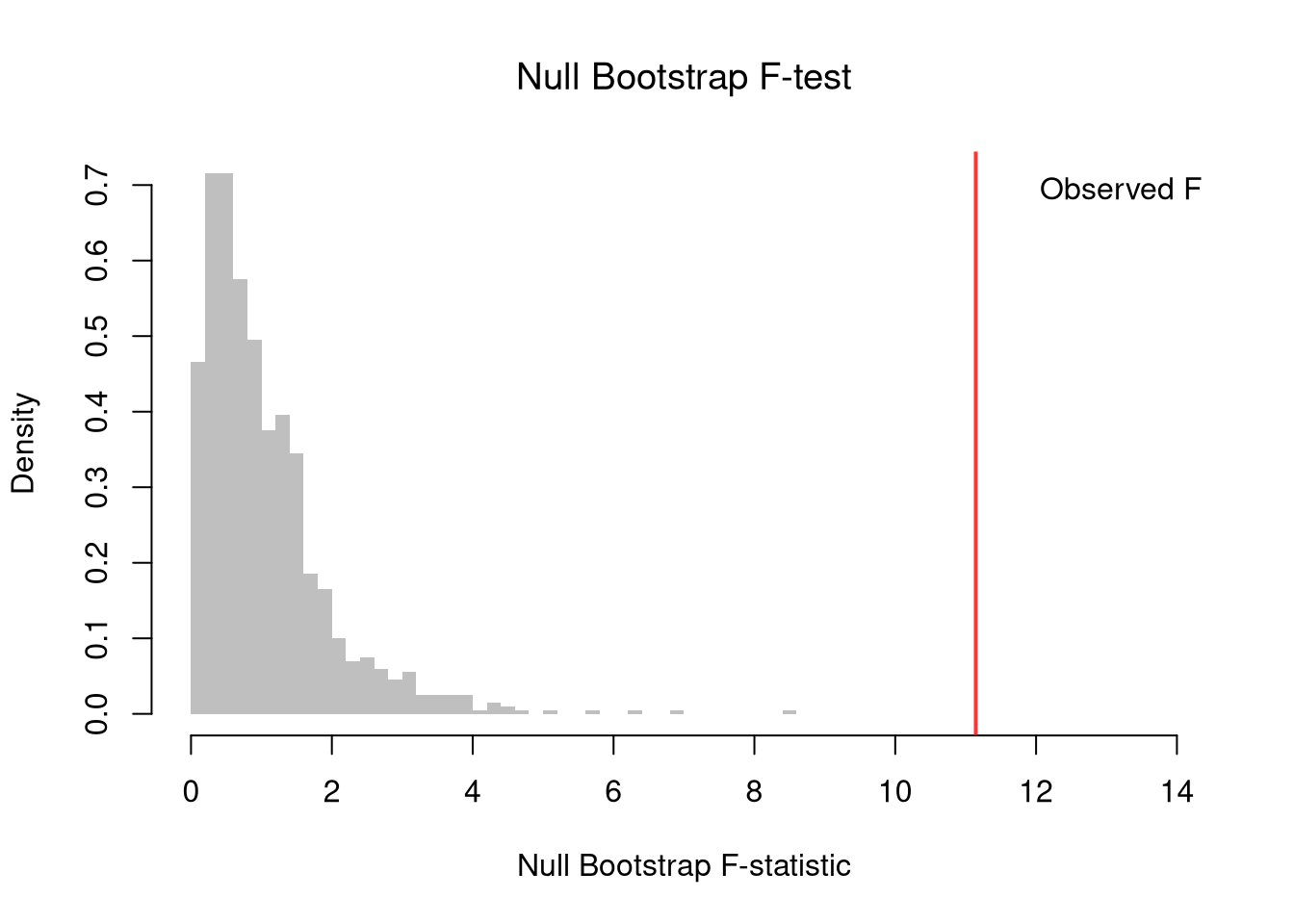
Under additional parametric assumptions (independent observations, equal variances, normal errors), \(\hat{F}\) (under the null) follows an \(F_{G-1,\;n-G}\) distribution. From that theoretical null distribution, we can then compute p-values (which is the default report method in R).
summary(fit_aov)
##             Df Sum Sq Mean Sq F value   Pr(>F)
## Region       3  391.2   130.4   11.14 1.28e-05 ***
## Residuals   46  538.3    11.7
## ---
## Signif. codes:  0 '***' 0.001 '**' 0.01 '*' 0.05 '.' 0.1 ' ' 1

p_param <- 1 - pf(F_obs, G-1, n-G)

 # Compare parametric and bootstrap p-values
cbind(F_obs, p_param, p_boot)
##         F_obs      p_param p_boot
## [1,] 11.14389 0.0001093623 0The Kruskal-Wallis test examines \(H_0:\; F_1 = F_2 = \dots = F_G\) versus \(H_A:\) at least one \(F_g\) differs, where \(F_g\) is the continuous distribution of group \(g=1,...G\). This test does not tell us which group is different.
To conduct the test, first denote individuals \(i=1,...n\) with overall ranks \(\hat{r}_1,....\hat{r}_{n}\). Each individual belongs to group \(g=1,...G\), and each group \(g\) has \(n_{g}\) individuals with average rank \(\bar{r}_{g} = \sum_{i} \hat{r}_{i} /n_{g}\). The Kruskal Wallis statistic is \[\begin{eqnarray} \hat{KW} &=& (n-1) \frac{\sum_{g=1}^{G} n_{g}( \bar{r}_{g} - \bar{r} )^2 }{\sum_{i=1}^{n} ( \hat{r}_{i} - \bar{r} )^2}, \end{eqnarray}\] where \(\bar{r} = \frac{n+1}{2}\) is the grand mean rank.
In the special case with only two groups, the Kruskal Wallis test reduces to the Mann–Whitney U test (also known as the Wilcoxon rank-sum test). In this case, we can write the hypotheses in terms of individual outcomes in each group, \(Y_i\) in one group \(Y_j\) in the other; \(H_0: Prob(Y_i > Y_j)=Prob(Y_i > Y_i)\) versus \(H_A: Prob(Y_i > Y_j) \neq Prob(Y_i > Y_j)\). The corresponding test statistic is \[\begin{eqnarray} \hat{U} &=& \min(\hat{U}_1, \hat{U}_2) \\ \hat{U}_g &=& \sum_{i\in g}\sum_{j\in -g} \Bigl[\mathbf 1( \hat{Y}_{i} > \hat{Y}_{j}) + \tfrac12\mathbf 1(\hat{Y}_{i} = \hat{Y}_{j})\Bigr]. \end{eqnarray}\]
Interpretation template:
kw <- kruskal.test(Murder ~ Region, data = dat)
kw
##
##  Kruskal-Wallis rank sum test
##
## data:  Murder by Region
## Kruskal-Wallis chi-squared = 19.345, df = 3, p-value = 0.000232ANOVA is a special case of linear regression where the only explanatory variables are group indicators.
The model \(\hat{Y}_{ig} = b_0 + \sum_{g=2}^{G} b_g \hat{D}_{ig} + e_{ig}\) produces the same F-statistic as above. Here \(b_0\) estimates the mean of the reference group and each \(b_g\) estimates the difference between group \(g\) and the reference.
# Compare to group means
M_g <- aggregate(Murder ~ Region, dat, mean)$Murder
M_g
## [1]  4.700000 11.706250  5.700000  7.030769

# b0 = mean of reference group; b_g = mean(g) - mean(reference)
M_g - M_g[1]
## [1] 0.000000 7.006250 1.000000 2.330769

# Regression coefficients = group mean differences
fit_lm <- lm(Murder ~ Region, data = dat)
coef(fit_lm)
##         (Intercept)         RegionSouth RegionNorth Central          RegionWest
##            4.700000            7.006250            1.000000            2.330769
As such, the ANOVA table for a regression with a single factor is the same as one for AOV.
anova(fit_aov)
## Analysis of Variance Table
##
## Response: Murder
##           Df Sum Sq Mean Sq F value    Pr(>F)
## Region     3 391.24 130.412  11.144 1.282e-05 ***
## Residuals 46 538.32  11.703
## ---
## Signif. codes:  0 '***' 0.001 '**' 0.01 '*' 0.05 '.' 0.1 ' ' 1
anova(fit_lm)
## Analysis of Variance Table
##
## Response: Murder
##           Df Sum Sq Mean Sq F value    Pr(>F)
## Region     3 391.24 130.412  11.144 1.282e-05 ***
## Residuals 46 538.32  11.703
## ---
## Signif. codes: 0 '***' 0.001 '**' 0.01 '*' 0.05 '.' 0.1 ' ' 1We can extend the group-comparison model by adding continuous predictors alongside the factor. For example, we might ask: after controlling for Assault, do regional differences in murder rates persist?
# Extend the model: add Assault as a continuous predictor
reg_combined <- lm(Murder ~ Region + Assault, data = dat)
summary(reg_combined)
##
## Call:
## lm(formula = Murder ~ Region + Assault, data = dat)
##
## Residuals:
##     Min      1Q  Median      3Q     Max
## -6.4434 -1.2104  0.0058  1.6280  6.0123
##
## Coefficients:
##                     Estimate Std. Error t value Pr(>|t|)
## (Intercept)         0.216516   0.936455   0.231 0.818201
## RegionSouth         3.702630   1.021206   3.626 0.000731 ***
## RegionNorth Central 1.224174   0.986690   1.241 0.221151
## RegionWest          0.187047   1.007021   0.186 0.853481
## Assault             0.035396   0.004474   7.912 4.63e-10 ***
## ---
## Signif. codes:  0 '***' 0.001 '**' 0.01 '*' 0.05 '.' 0.1 ' ' 1
##
## Residual standard error: 2.237 on 45 degrees of freedom
## Multiple R-squared:  0.7578, Adjusted R-squared:  0.7363
## F-statistic:  35.2 on 4 and 45 DF,  p-value: 2.511e-13
With factors, you can still include them in the design matrix of an OLS regression. For example, \[\begin{eqnarray} \hat{Y}_{i} = \sum_{k=0}^{K} b_k \hat{X}_{ik} + \sum_{g}\hat{D}_{g}b_{g} \end{eqnarray}\] When, as commonly done, the factors are modeled as being additively separable, they are modeled as fixed effects.1 Simply including the factors into the OLS regression yields a “dummy variable” fixed effects estimator. The fixed effects and dummy variable approach are algebraically equal: same coefficients and same residuals. (See Hansen Econometrics, Theorem 17.1)
# Dummy variable approach
reg_dv <- lm(Murder ~ -1 + Assault + Region, data = dat)
coef(reg_dv)['Assault']
##    Assault
## 0.03539592

# Fixed effects approach
library(fixest)
reg_fe <- feols(Murder ~ Assault | Region, data = dat)
coef(reg_fe)
##    Assault
## 0.03539592
With fixed effects, we can also compute averages for each group: \(\hat{M}_{Yg}=\sum_{i}^{n_{g}} \hat{Y}_{ig}/n_{g}\), where each group \(g\) has \(n_{g}\) observations denoted \(\hat{Y}_{ig}\). We can then construct a between estimator: \(\hat{M}_{Yg} = b_{0} + \hat{M}_{Xg} b_{1}\). Or we can subtract the average from each group to construct a within estimator: \((\hat{Y}_{ig} - \hat{M}_{Yg}) = (\hat{X}_{ig}-\hat{M}_{Xg})b_{1}\).
Recall that we can compare regression models using an F-Test. Under some additional parametric assumptions, the F-statistic follows an \(F\) distribution. This case is well-studied historically under the title Analysis of Variance (ANOVA). We can build a sequence of nested models to see which predictors contribute.
# Sequence of nested models
reg0 <- lm(Murder ~ 1, data = dat)               # intercept only
reg1 <- lm(Murder ~ Region, data = dat)           # Region (the ANOVA model)
reg2 <- lm(Murder ~ Region + Assault, data = dat) # Region + Assault
reg3 <- lm(Murder ~ Region * Assault, data = dat) # Region * Assault

# Does Region explain murder rates?
anova(reg0, reg1)
## Analysis of Variance Table
##
## Model 1: Murder ~ 1
## Model 2: Murder ~ Region
##   Res.Df    RSS Df Sum of Sq      F    Pr(>F)
## 1     49 929.55
## 2     46 538.32  3    391.24 11.144 1.282e-05 ***
## ---
## Signif. codes:  0 '***' 0.001 '**' 0.01 '*' 0.05 '.' 0.1 ' ' 1

# Does adding Assault improve the model beyond Region?
anova(reg1, reg2)
## Analysis of Variance Table
##
## Model 1: Murder ~ Region
## Model 2: Murder ~ Region + Assault
##   Res.Df    RSS Df Sum of Sq      F    Pr(>F)
## 1     46 538.32
## 2     45 225.12  1    313.19 62.605 4.626e-10 ***
## ---
## Signif. codes:  0 '***' 0.001 '**' 0.01 '*' 0.05 '.' 0.1 ' ' 1

# Does the effect of Assault differ by Region?
anova(reg2, reg3)
## Analysis of Variance Table
##
## Model 1: Murder ~ Region + Assault
## Model 2: Murder ~ Region * Assault
##   Res.Df    RSS Df Sum of Sq     F Pr(>F)
## 1     45 225.12
## 2 42 212.05 3 13.072 0.863 0.4678# Manual F-test: intercept-only vs Region
rss0 <- sum(resid(reg0)^2)
rss1 <- sum(resid(reg1)^2)
df0 <- df.residual(reg0)
df1 <- df.residual(reg1)
F <- ((rss0 - rss1)/(df0 - df1)) / (rss1/df1)
p <- 1 - pf(F, df0 - df1, df1)
cbind(F, p)
## F p
## [1,] 11.14389 1.282093e-05An ANOVA \(F\)-test rejects the null that all group means are equal. Does this tell you which group is different, or only that at least one differs?
Using the USArrests dataset with state.region as the grouping variable, compute the between-group sum of squares (\(\hat{BSS}\)) and within-group sum of squares (\(\hat{WSS}\)) for Assault by hand (using aggregate()). Verify your \(\hat{F}\) statistic matches the output of summary(aov(Assault ~ state.region, data = ...)).
Extend the running example by fitting Murder ~ Region + Assault + UrbanPop and Murder ~ Region * Assault + UrbanPop. Use anova() to test whether the Region-Assault interaction terms are jointly significant after controlling for UrbanPop. Compare your conclusion to the interaction test without UrbanPop shown in the chapter.
There are also random effects: the factor variable comes from a distribution that is uncorrelated with the regressors. This is rarely used in economics today, however, and are mostly included for historical reasons and special cases where fixed effects cannot be estimated due to data limitations.↩︎