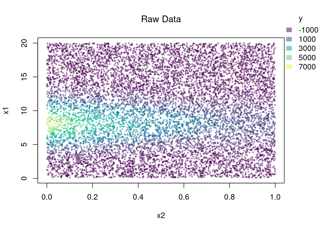
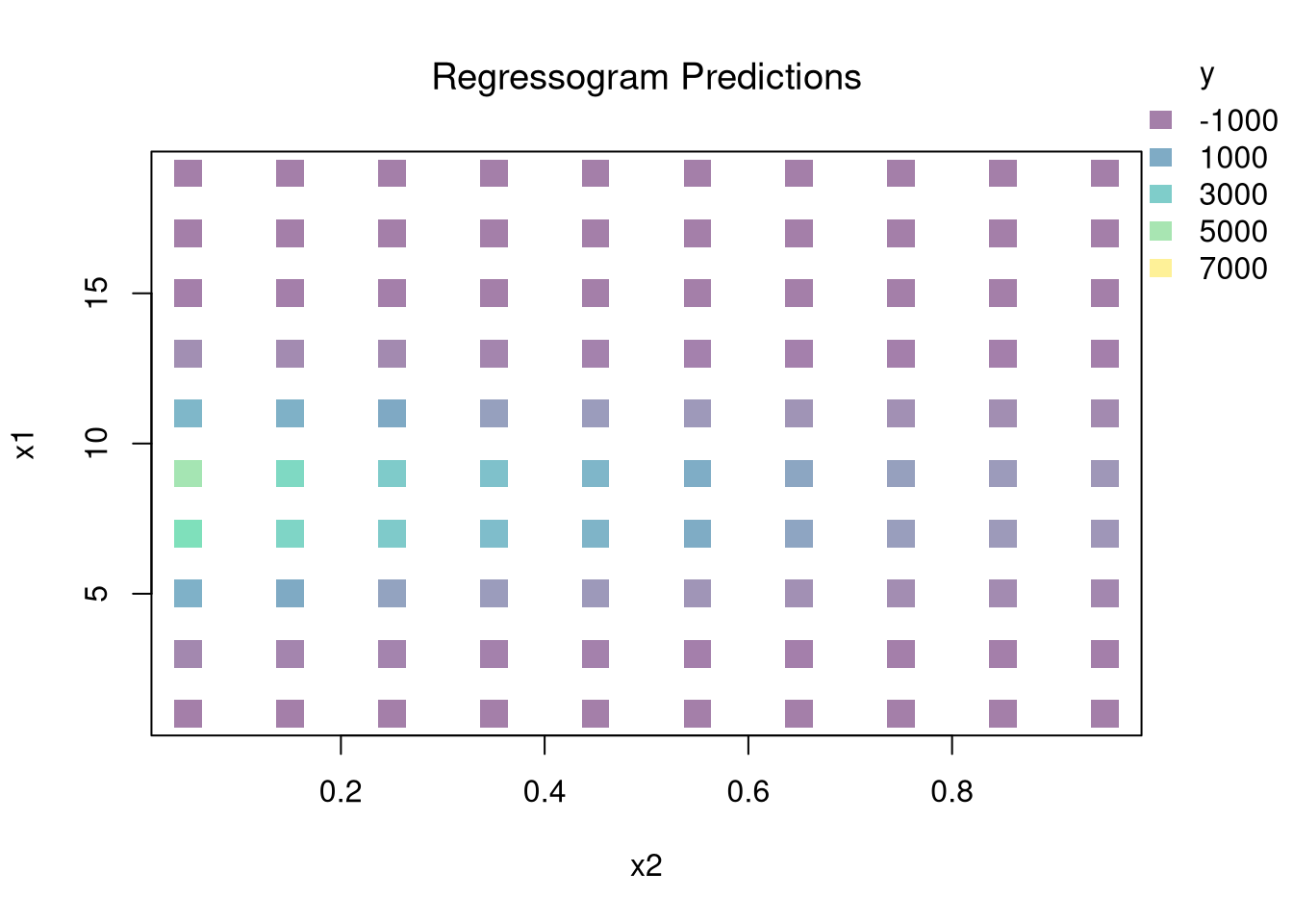
You can estimate a nonparametric model with multiple \(X\) variables with a multivariate regressogram. Here, we cut the data into exclusive bins along each dimension (called dummy variables), and then run a regression on all dummy variables.
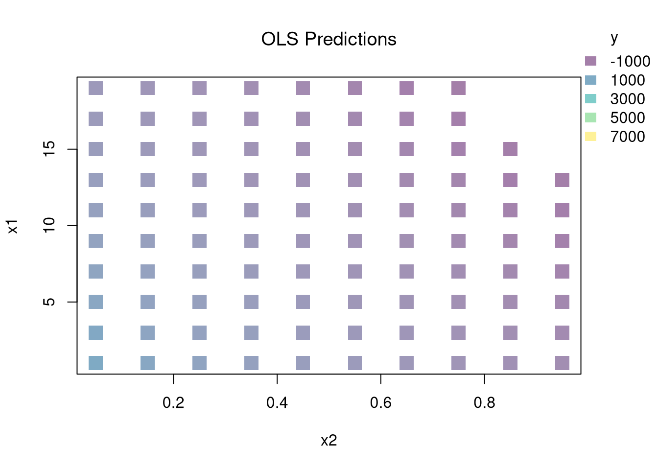
The regressogram divides the \((x_1, x_2)\) space into a grid of bins and estimates the mean of \(y\) within each bin. Compared to OLS, the regressogram makes no assumption about functional form: it can capture nonlinear and interaction effects. The trade-off is that it requires more data to fill each bin, especially as the number of variables grows.
22.2 Local Regressions
Just like with bivariate data, you can also use split-sample (or piecewise) regressions for multivariate data.
Break Points.
Incorporating Kinks and Discontinuities in \(X\) are a type of transformation that can be modeled using factor variables. As such, \(F\)-tests can be used to examine whether a breaks is statistically significant.
Code
library(Ecdat)reg <-lm(wage ~ school, data=Wages1)# F Test for Breakreg2 <-lm(wage ~ school*I(school>12), data=Wages1)anova(reg, reg2)# Chow Test for Breakdata_splits <-split(Wages1, Wages1$school <=12)resids <-sapply(data_splits, function(dat){ reg <-lm(wage ~ school, data=dat)sum( resid(reg)^2)})Ns <-sapply(data_splits, function(dat){ nrow(dat)})Rt <- (sum(resid(reg)^2) -sum(resids))/sum(resids)Rb <- (sum(Ns)-2*reg$rank)/reg$rankFt <- Rt*Rbpf(Ft, reg$rank, sum(Ns)-2*reg$rank, lower.tail=F)# See also# strucchange::sctest(y ~ x, data=xy, type='Chow', point=.5)# strucchange::Fstats(y ~ x, data=xy)# To Find Changes# segmented::segmented(reg)
NoteMust Know
The Chow test checks whether a structural break exists at a specified point. What happens if you do not know where the break is? How does searching over many potential break points affect the validity of your test? (Hint: think about multiple testing.)
22.3 Model Selection
One of the most common approaches to selecting a model or bandwidth is to minimize error. Leave-one-out Cross-validation minimizes the average “leave-one-out” mean square prediction errors: \[\begin{eqnarray}
\min_{\mathbf{H}} \quad \frac{1}{n} \sum_{i=1}^{n} \left[ \hat{Y}_{i} - \hat{y_{[i]}}(\mathbf{X},\mathbf{H}) \right]^2,
\end{eqnarray}\] where \(\hat{y}_{[i]}(\mathbf{X},\mathbf{H})\) is the model predicted value at \(\mathbf{X}_{i}\) based on a dataset that excludes \(\mathbf{X}_{i}\), and \(\mathbf{H}\) is matrix of bandwidths. With a weighted least squares regression on three explanatory variables, for example, the matrix is \[\begin{eqnarray}
\mathbf{H}=\begin{pmatrix}
h_{1} & 0 & 0 \\
0 & h_{2} & 0 \\
0 & 0 & h_{3} \\
\end{pmatrix},
\end{eqnarray}\] where each \(h_{k}\) is the bandwidth for variable \(X_{k}\).
There are many types of cross-validation (ArlotCelisse2010?; BatesEtAl2023?). For example, one extension is k-fold cross validation, which splits \(N\) datapoints into \(k=1...K\) groups, each sized \(B\), and predicts values for the left-out group. adjusts for the degrees of freedom, whereas the function in R uses (racine2019?) by default. You can refer to extensions on a case by case basis.
TipTest Yourself
Cross-validation works by repeatedly holding out one observation, fitting the model on the rest, and measuring how well the model predicts the held-out point. A model that overfits (e.g., too many bins) will have low in-sample error but high cross-validation error. The bandwidth \(\mathbf{H}\) that minimizes cross-validation error balances flexibility against overfitting.
22.4 Hypothesis Testing
There are two main ways to summarize gradients: how \(Y\) changes with \(X\).
For regressograms, you can approximate gradients with small finite differences. For some small \(h_{p}\), we can compute \[\begin{eqnarray}
\hat{\beta}_{p}(\mathbf{x}) &=& \frac{ \hat{y}(x_{1},...,x_{p}+ \frac{h_{p}}{2}...,x_{P})-\hat{y}(x_{1},...,x_{p}-\frac{h_{p}}{2}...,x_{P})}{h_{p}},
\end{eqnarray}\]
When using split-sample regressions or local linear regressions, you can use the estimated slope coefficients \(\hat{\beta}_{p}(\mathbf{x})\) as gradient estimates in each direction.
After computing gradients, you can summarize them in various plots: Histogram of \(\hat{\beta}_{p}(\mathbf{x})\), Scatterplot of \(\hat{\beta}_{p}(\mathbf{x})\) vs. \(X_{p}\), or the CI of \(\hat{\beta}_{p}(\mathbf{x})\) vs \(\hat{\beta}_{p}(\mathbf{x})\) after sorting the gradients (Chaudhuri1999?; HendersonEtAl2012?)
You may also be interested in a particular gradient or a single summary statistic. For example, a bivariate regressogram can estimate the marginal effect of \(X_{1}\) at the means; \(\hat{\beta_{1}}(\bar{\mathbf{x}}=[\bar{x_{1}}, \bar{x_{2}}])\). You may also be interested in the mean of the marginal effects (sometimes said simply as “average effect”), which averages the marginal effect over all datapoints in the dataset: \(1/n \sum_{i}^{n} \hat{\beta_{1}}(\mathbf{X}_{i})\), or the median marginal effect. Such statistics are single numbers that can be presented similar to an OLS regression table where each row corresponds a variable and each cell has two elements: “mean gradient (sd gradient)”.
22.5 Exercises
A regressogram bins each explanatory variable and estimates a separate mean within each bin combination. How does this differ from a standard OLS regression with the same variables? What advantage does it have when the true relationship is nonlinear, and what is its main drawback as the number of explanatory variables grows?
Using the simulated data from this chapter (x1 <- seq(.1, 20, length.out = 1000), x2 <- runif(1000, 0, 1), y <- 3*exp(-2*x2 + 1.5*x1 - .1*x1^2)*x1 + rnorm(1000)), build a regressogram by cutting x1 into 5 bins and x2 into 5 bins. Compute the mean of y within each of the 25 bin combinations. Which bin combination has the highest predicted value?
Using lm(), fit two models to the mtcars dataset with mpg as the outcome: (a) a standard linear model mpg ~ wt + hp, and (b) a regressogram model where wt and hp are each cut into 4 bins using cut() and interacted (mpg ~ cut(wt,4) * cut(hp,4)). Compare the \(\hat{R}^2\) of each model. Plot the predicted values from both models against the observed mpg.