In practice, it is hard to find a good natural experiment and easy to find a bad one. Paradoxically, natural experiments are something you are supposed to find but never search for. As you search for natural experiments, sometimes patterns will appear from random noise. In this age of big data, we are getting increasingly more data and, perhaps surprisingly, this makes it easier to make false discoveries. This chapter examines how those discoveries arise, first through three classical routes (data errors, \(p\)-hacking, and spurious regression), and then through the latest and greatest empirical recipes (IV, RDD, DID) applied to data that is nothing but noise. Although it is difficult to express numerically, searching for a good natural experiment can also lead you astray from important questions. There are good reasons to be excited about empirical social science, but we would be wise to recall some earlier wisdom from economists on the matter.
The most reckless and treacherous of all theorists is he who professes to let facts and figures speak for themselves, who keeps in the background the part he has played, perhaps unconsciously, in selecting and grouping them
— Alfred Marshall, 1885
The blind transfer of the striving for quantitative measurements to a field where the specific conditions are not present which give it its basic importance in the natural sciences is the result of an entirely unfounded prejudice. It is probably responsible for the worst aberrations and absurdities produced by scientism in the social sciences. It not only leads frequently to the selection for study of the most irrelevant aspects of the phenomena because they happen to be measurable, but also to “measurements” and assignments of numerical values which are absolutely meaningless. What a distinguished philosopher recently wrote about psychology is at least equally true of the social sciences, namely that it is only too easy “to rush off to measure something without considering what it is we are measuring, or what measurement means. In this respect some recent measurements are of the same logical type as Plato’s determination that a just ruler is 729 times as happy as an unjust one.”
— F.A. Hayek, 1943
if you torture the data long enough, it will confess
— R. Coase (Source Unknown)
the definition of a causal parameter is not always clearly stated, and formal statements of identifying conditions in terms of well-specified economic models are rarely presented. Moreover, the absence of explicit structural frameworks makes it difficult to cumulate knowledge across studies conducted within this framework. Many studies produced by this research program have a `stand alone’ feature and neither inform nor are influenced by the general body of empirical knowledge in economics.
— J.J. Heckman, 2000
without explicit prior consideration of the effect of the instrument choice on the parameter being estimated, such a procedure is effectively the opposite of standard statistical practice in which a parameter of interest is defined first, followed by an estimator that delivers that parameter. Instead, we have a procedure in which the choice of the instrument, which is guided by criteria designed for a situation in which there is no heterogeneity, is implicitly allowed to determine the parameter of interest. This goes beyond the old story of looking for an object where the light is strong enough to see; rather, we have at least some control over the light but choose to let it fall where it may and then proclaim that whatever it illuminates is what we were looking for all along.
— A. Deaton, 2010
False Discoveries
False Discovery.
Modern research generates so many statistical tests that some “significant” findings appear by chance alone, even when no real effect exists.
A false discovery is a statistically significant result that does not reflect a true effect in the population.
False discoveries are useful to track because their rate is what classical hypothesis tests claim to control: a 5% test promises a 5% false-discovery rate on null data, and any procedure that raises this rate above the stated level (whether through search, dependence, or sloppy data) inflates the headline number. The three engines surveyed below: data errors, \(p\)-hacking, and spurious regression, all generate false discoveries without anyone behaving fraudulently.
Data Errors.
A huge amount of data normally means a huge amount of data cleaning/merging/aggregating. This avoids many copy-paste errors, which are a recipe for disaster, but may also introduce other types of errors. Some spurious results are driven by honest errors in data cleaning. According to one estimate, this is responsible for around one fifth of all medical science retractions (there is even a whole book about this!). Although there are not similar meta-analysis in economics, there are some high-profile examples. This includes papers that are highly influential, like Lott, Levitt and Reinhart and Rogoff as well as others the top economics journals, like the RESTUD and AER. There are some reasons to think such errors are more widespread across the social sciences; e.g., in Census data and Aid data. So be careful!
Note: one reason to plot your data is to help spot such errors. Data errors are only one route to a spurious finding. The next one is searching the same dataset for any specification that “works”.
P-Hacking.
Once you can run dozens of regressions in a single afternoon, the search for “significance” itself becomes a route to false discoveries that no single \(p\)-value can warn you about.
P-hacking is the practice of trying many models, transformations, or subsamples and then reporting a \(p\)-value that does not account for those searches (no longer reflecting the true probability of seeing the result under the null).
P-hacking is useful to recognize because it can occur without any fraudulent intent: trying different variable transformations or sample windows to uncover patterns is itself a form of search. Its various synonyms (data drudging, star mining) name the same behavior across different disciplines. The practice is both pernicious and widespread, and applies equally to OLS and to more sophisticated tools like 2SLS, as the next two code blocks illustrate.
Code
# P-hacking OLS with different explanatory vars
set.seed(123)
n <- 50
X1 <- runif(n)

# Regression Machine:
# repeatedly finds covariate, runs regression
# stops when statistically significant at .1%
p <- 1
i <- 0
while(p >= .001){
    # Get Random Covariate
    X2 <-  runif(n)
    # Merge and `Analyze'
    dat_i <- data.frame(X1, X2)
    reg_i <- lm(X1 ~ X2, data=dat_i)
    # update results in global environment
    p <- summary(reg_i)$coefficients[2, 4]
    i <- i+1
}
#summary(reg_i)

plot(X1 ~ X2, data=dat_i,
    pch=16, col=grey(0, .5), main=NA)
title(paste0('Random Dataset ', i, ':   p=',
    formatC(p, digits=2, format='fg')), font.main=1)
abline(reg_i, col=rgb(1, 0, 0, .8))
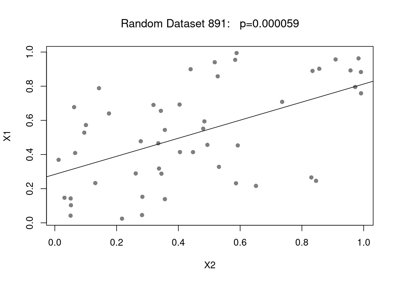
The loop ran through i random datasets before finding one with \(p < 0.001\). With truly random data, each regression has a \(0.1\%\) chance of producing \(p < 0.001\). After \(k\) independent tests, the probability of at least one false discovery is \(1-(1-\alpha)^k\). The probability climbs fast in \(k\):
Code
alpha <- 0.001
k <- c(1, 10, 100, 700, 5000)
round(1 - (1 - alpha)^k, 3)
## [1] 0.001 0.010 0.095 0.504 0.993
So at \(k=700\) tries the chance of at least one false discovery exceeds 50%, and by \(k=5000\) it is essentially 1. The more you search, the more likely you are to find a spurious result. See Multiple Testing in the next chapter for corrections that control this family-wise error rate.
Code
# P-hacking 2SLS with different explanatory vars
# and different instrumental vars
library(fixest)
p <- 1
ii <- 0
set.seed(123)
while(p >= .05){
    # Get Random Covariates
    X2 <-  runif(n)
    X3 <-  runif(n)
    # Create Treatment Variable based on Cutoff
    cutoffs <- seq(0, 1, length.out=11)[-c(1, 11)]
    for(tau in cutoffs){
        T3 <- 1*(X3 > tau)
        # Merge and `Analyze'
        dat_i <- data.frame(X1, X2, T3)
        ivreg_i <- feols(X1 ~ 1|X2 ~ T3, data=dat_i)
        # Update results in global environment
        ptab <- summary(ivreg_i)$coeftable
        if( nrow(ptab)==2){
            p <- ptab[2, 4]
            ii <- ii+1
        }
    }
}
summary(ivreg_i)
## TSLS estimation: Second stage
## |- D.V.   : X1
## |- Endo.  : X2
## |- Instr. : T3
## Dep. Var.: X1
## Observations: 50
## Standard-errors: IID
##              Estimate Std. Error       t value  Pr(>|t|)
## (Intercept) -1.07e-13   1.21e-13 -8.850710e-01   0.38053
## fit_X2       1.00e+00   2.33e-13  4.294143e+12 < 2.2e-16 ***
## ---
## Signif. codes:  0 '***' 0.001 '**' 0.01 '*' 0.05 '.' 0.1 ' ' 1
## RMSE: 5.494e-14   Adj. R2: -0.006886
## F-test (1st stage), X2: stat = 0.66488, p = 0.418869, on 1 and 48 DoF.
##             Wu-Hausman: stat = 0.12881, p = 0.721276, on 1 and 47 DoF.
The p-hacking example found a statistically significant IV result using random data. What safeguards could a researcher adopt to avoid this problem? Consider: (a) pre-registration of hypotheses, (b) adjusting for multiple testing, and (c) out-of-sample validation.
Spurious Regression
Even without any coding errors or p-hacking, you can sometimes make a false discovery. We begin with a motivating empirical example of “US Gov’t Spending on Science”.
Trending Series.
When two variables both drift upward over time, OLS can flag them as related even when nothing connects them.
Spurious regression arises when two unrelated time series share a common trend and so produce a large \(\hat{R}^2\) and a small \(p\)-value when one is regressed on the other.
Spurious regression is useful to know about because the resulting significance is not a property of any underlying relationship. It grows with the sample length, so longer time series make the problem worse rather than better. The mechanism is a violation of the OLS independence assumption: the standard errors assume independent observations, and trending series share so much information across periods that the effective sample size is far smaller than \(n\).
First, get and inspect some data from https://tylervigen.com/spurious-correlations
Code
# Your data is not made up in the computer (hopefully!)
vigen_csv <- read.csv(
    'https://raw.githubusercontent.com/the-mad-statter/whysospurious/master/data-raw/tylervigen.csv'
)
class(vigen_csv)
## [1] "data.frame"
names(vigen_csv)
##  [1] "year"                         "science_spending"
##  [3] "hanging_suicides"             "pool_fall_drownings"
##  [5] "cage_films"                   "cheese_percap"
##  [7] "bed_deaths"                   "maine_divorce_rate"
##  [9] "margarine_percap"             "miss_usa_age"
## [11] "steam_murders"                "arcade_revenue"
## [13] "computer_science_doctorates"  "noncom_space_launches"
## [15] "sociology_doctorates"         "mozzarella_percap"
## [17] "civil_engineering_doctorates" "fishing_drownings"
## [19] "kentucky_marriage_rate"       "oil_imports_norway"
## [21] "chicken_percap"               "train_collision_deaths"
## [23] "oil_imports_total"            "pool_drownings"
## [25] "nuclear_power"                "japanese_cars_sold"
## [27] "motor_vehicle_suicides"       "spelling_bee_word_length"
## [29] "spider_deaths"                "math_doctorates"
## [31] "uranium"
vigen_csv[1:5, 1:5]
##   year science_spending hanging_suicides pool_fall_drownings cage_films
## 1 1996               NA               NA                  NA         NA
## 2 1997               NA               NA                  NA         NA
## 3 1998               NA               NA                  NA         NA
## 4 1999            18079             5427                 109          2
## 5 2000            18594             5688                 102          2
Examine some data
Code
par(mfrow=c(1, 2), mar=c(2, 2, 2, 1))
plot.new()
plot.window(xlim=c(1999, 2009), ylim=c(5, 9)*1000)
lines(science_spending/3 ~ year, data=vigen_csv, lty=1, col=rgb(1, 0, 0, .8), pch=16)
text(2003, 8200, 'US spending on science, space, technology (USD/3)', col=rgb(1, 0, 0, .8), cex=.6, srt=30)
lines(hanging_suicides ~ year, data=vigen_csv, lty=1, col=rgb(0, 0, 1, .8), pch=16)
text(2004, 6500, 'US Suicides by hanging, strangulation, suffocation (Deaths)', col=rgb(0, 0, 1, .8), cex=.6, srt=30)
axis(1)
axis(2)


plot.new()
plot.window(xlim=c(2002, 2009), ylim=c(0, 5))
lines(cage_films ~ year, data=vigen_csv[vigen_csv$year>=2002, ], lty=1, col=rgb(1, 0, 0, .8), pch=16)
text(2006, 0.5, 'Number of films with Nicolas Cage (Films)', col=rgb(1, 0, 0, .8), cex=.6, srt=0)
lines(pool_fall_drownings/25 ~ year, data=vigen_csv[vigen_csv$year>=2002, ], lty=1, col=rgb(0, 0, 1, .8), pch=16)
text(2006, 4.5, 'Number of drownings by falling into pool (US Deaths/25)', col=rgb(0, 0, 1, .8), cex=.6, srt=0)
axis(1)
axis(2)
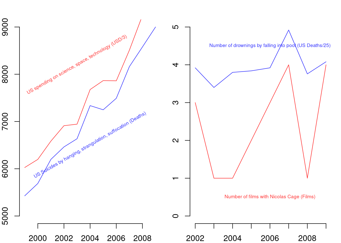
Both plots show variables with high correlations (\(r > 0.9\)) that have no causal connection. The correlations arise because both series trend upward over time. When two time series share a common trend, their correlation can be very high even if they are completely unrelated. This is why regression with trending time series requires special care (e.g., detrending or differencing).
Another Example.
The US government spending on science is ruining cinema (p<.001)!?
Code
# Drop Data before 1999
vigen_csv <- vigen_csv[vigen_csv$year >= 1999, ]

# Run OLS Regression of Cage's film count on science spending.
# The p-value on `science_spending` will be tiny, despite zero plausible causal link.
reg1 <-  lm(cage_films ~ -1 + science_spending, data=vigen_csv)
summary(reg1)
##
## Call:
## lm(formula = cage_films ~ -1 + science_spending, data = vigen_csv)
##
## Residuals:
##     Min      1Q  Median      3Q     Max
## -1.7670 -0.7165  0.1447  0.7890  1.4531
##
## Coefficients:
##                   Estimate Std. Error t value Pr(>|t|)
## science_spending 9.978e-05  1.350e-05    7.39 2.34e-05 ***
## ---
## Signif. codes:  0 '***' 0.001 '**' 0.01 '*' 0.05 '.' 0.1 ' ' 1
##
## Residual standard error: 1.033 on 10 degrees of freedom
##   (1 observation deleted due to missingness)
## Multiple R-squared:  0.8452, Adjusted R-squared:  0.8297
## F-statistic: 54.61 on 1 and 10 DF,  p-value: 2.343e-05
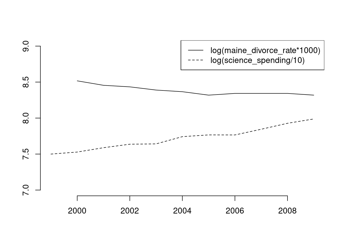
It’s not all bad, because people in Maine stay married longer?
Code
plot.new()
plot.window(xlim=c(1999, 2009), ylim=c(7, 9))
lines(log(maine_divorce_rate*1000) ~ year, data=vigen_csv)
lines(log(science_spending/10) ~ year, data=vigen_csv, lty=2)
axis(1)
axis(2)
legend('topright', lty=c(1, 2), bty='n', legend=c(
    'log(maine_divorce_rate*1000)',
    'log(science_spending/10)'))
For more intuition on spurious correlations, try http://shiny.calpoly.sh/Corr_Reg_Game/ The same principles apply to more sophisticated methods.
Spurious Causal Impacts
Good natural experiments are hard to find. For example, suppose we asked “what is the effect of wages on police demanded?” and examined a policy which lowered the educational requirements from 4 years to 2 to become an officer. This increases the labour supply, but it also affects the demand curve through “general equilibrium”: as some of the new officers were potentially criminals and, with fewer criminals, the demand for police shifts down. Bad natural experiments, by contrast, are easier to find than you might imagine. The remainder of this section illustrates that risk: applying canonical causal-inference recipes (IV, RDD, DID) to data that is purely noise.
Spurious Instrument.
The same search problem that produces spurious OLS results also produces spurious instruments. By chance, some candidate variable will satisfy the statistical tests for relevance and exogeneity.
A spurious instrument is a variable that satisfies the formal statistical criteria for an instrumental variable (relevance, exogeneity) by chance, despite having no plausible causal connection to the endogenous regressor.
A spurious instrument is useful to recognize because it is the IV analog of p-hacking: search over enough candidate instruments and one will pass the formal tests by luck, but the 2SLS estimate it produces has no causal interpretation. The risk grows with the number of candidates considered, which is the same multiple-testing problem as p-hacking applied to instrument selection. The Vigen IV exercise below shows this directly: most random variable triples in the spurious-correlations dataset return “significant” results at conventional levels.
Example: Vigen IV’s.
We now run IV regressions for different variable combinations in the dataset of spurious relationships
Code
knames <- names(vigen_csv)[2:11] # First 10 Variables
#knames <- names(vigen_csv)[-1] # Try All Variables
p <- 1
ii <- 1
ivreg_list <- vector('list', factorial(length(knames))/factorial(length(knames)-3))

# Choose 3 variable
for( k1 in knames){
for( k2 in setdiff(knames, k1)){
for( k3 in setdiff(knames, c(k1, k2)) ){
    X1 <- vigen_csv[, k1]
    X2 <- vigen_csv[, k2]
    X3 <- vigen_csv[, k3]
    # Merge and `Analyze'
    dat_i <- na.omit(data.frame(X1, X2, X3))
    ivreg_i <- feols(X1 ~ 1|X2 ~ X3, data=dat_i)
    ivreg_list[[ii]] <- list(ivreg_i, c(k1, k2, k3))
    ii <- ii+1
}}}
pvals <- sapply(ivreg_list, function(ivreg_i){ivreg_i[[1]]$coeftable[2, 4]})

plot(ecdf(pvals), xlab='p-value', ylab='CDF', main=NA)
title('Frequency IV is Statistically Significant', font.main=1)
abline(v=c(.01, .05), col=c(rgb(1, 0, 0, .8), rgb(0, 0, 1, .8)))
Code
# Most Significant Spurious Combinations
pvars <- sapply(ivreg_list, function(ivreg_i){ivreg_i[[2]]})
pdat <- data.frame(t(pvars), pvals)
pdat <- pdat[order(pdat$pvals), ]
head(pdat)
##                     X1                 X2            X3        pvals
## 76    hanging_suicides   science_spending    bed_deaths 3.049883e-08
## 4     science_spending   hanging_suicides    bed_deaths 3.049883e-08
## 3     science_spending   hanging_suicides cheese_percap 3.344890e-08
## 75    hanging_suicides   science_spending cheese_percap 3.344890e-08
## 485 maine_divorce_rate   margarine_percap cheese_percap 3.997738e-08
## 557   margarine_percap maine_divorce_rate cheese_percap 3.997738e-08

# Fraction of all combinations significant at conventional levels
c(at_0.05 = mean(pvals < 0.05, na.rm=TRUE),
  at_0.01 = mean(pvals < 0.01, na.rm=TRUE))
##   at_0.05   at_0.01
## 0.3166667 0.2194444
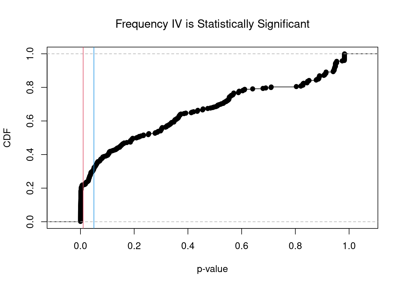
A noticeable share of the random variable triples returns “significant” results at both the 5% and 1% levels. That is far more than the rates a single hypothesis test would imply.
Simulation Study.
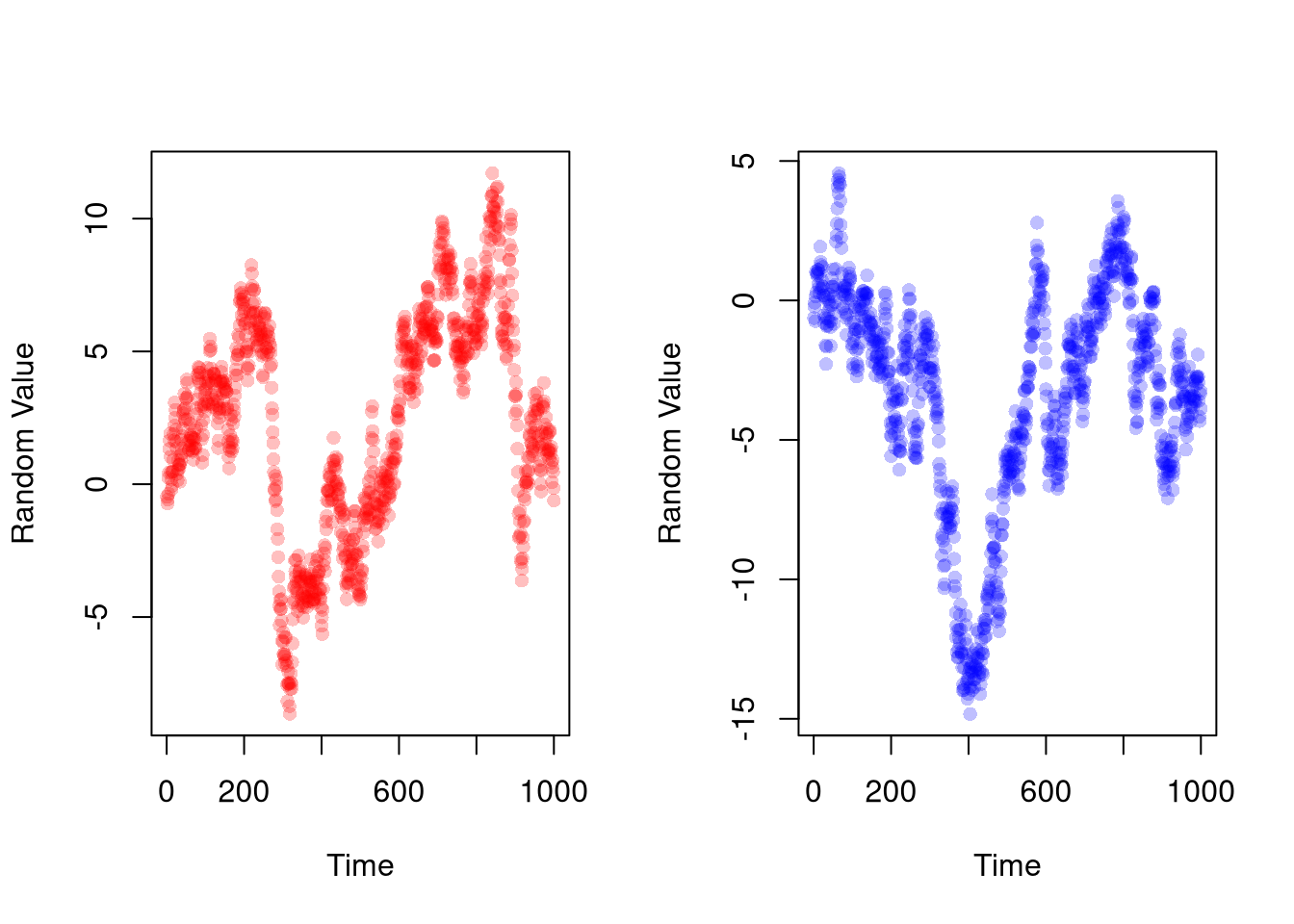
We do not have many theoretical results for these newer recipes yet, but a numerical example should make the issue clear. We apply the three major credible methods (IV, RDD, DID) to random walks. Each time, we find a result that fits mold and add various extensions that make it appear robust. One could tell a story about how \(X_{2}\) affects \(X_{1}\) but \(X_{1}\) might also affect \(X_{2}\), and how they discovered an instrument \(X_{3}\) to provide the first causal estimate of \(X_{2}\) on \(X_{1}\). The analysis looks scientific and the story sounds plausible, so you could probably be convinced if it were not just random noise.
Code
n <- 1000
n_index <- seq(n)

set.seed(1)
random_walk1 <- cumsum(runif(n, -1, 1))

set.seed(2)
random_walk2 <- cumsum(runif(n, -1, 1))

par(mfrow=c(1, 2))
plot(random_walk1, pch=16, col=rgb(1, 0, 0, .25),
    xlab='Time', ylab='Random Value')
plot(random_walk2, pch=16, col=rgb(0, 0, 1, .25),
    xlab='Time', ylab='Random Value')
IV. First, find an instrument that satisfy various statistical criterion to provide a causal estimate of \(X_{2}\) on \(X_{1}\).
Code
# 'Find' 'valid' ingredients
library(fixest)
random_walk3 <- cumsum(runif(n, -1, 1))
dat_i <- data.frame(
    X1=random_walk1,
    X2=random_walk2,
    X3=random_walk3)
ivreg_i <- feols(X1 ~ 1|X2 ~ X3, data=dat_i)
summary(ivreg_i)
## TSLS estimation: Second stage
## |- D.V.   : X1
## |- Endo.  : X2
## |- Instr. : X3
## Dep. Var.: X1
## Observations: 1,000
## Standard-errors: IID
##             Estimate Std. Error t value   Pr(>|t|)
## (Intercept)  8.53309   1.644285 5.18954 2.5533e-07 ***
## fit_X2       1.79901   0.472285 3.80916 1.4796e-04 ***
## ---
## Signif. codes:  0 '***' 0.001 '**' 0.01 '*' 0.05 '.' 0.1 ' ' 1
## RMSE: 6.25733   Adj. R2: 0.032314
## F-test (1st stage), X2: stat = 10.804, p = 0.001048, on 1 and 998 DoF.
##             Wu-Hausman: stat = 23.407, p = 1.518e-6, on 1 and 997 DoF.

# After experimenting with different instruments
# you can find even stronger results!
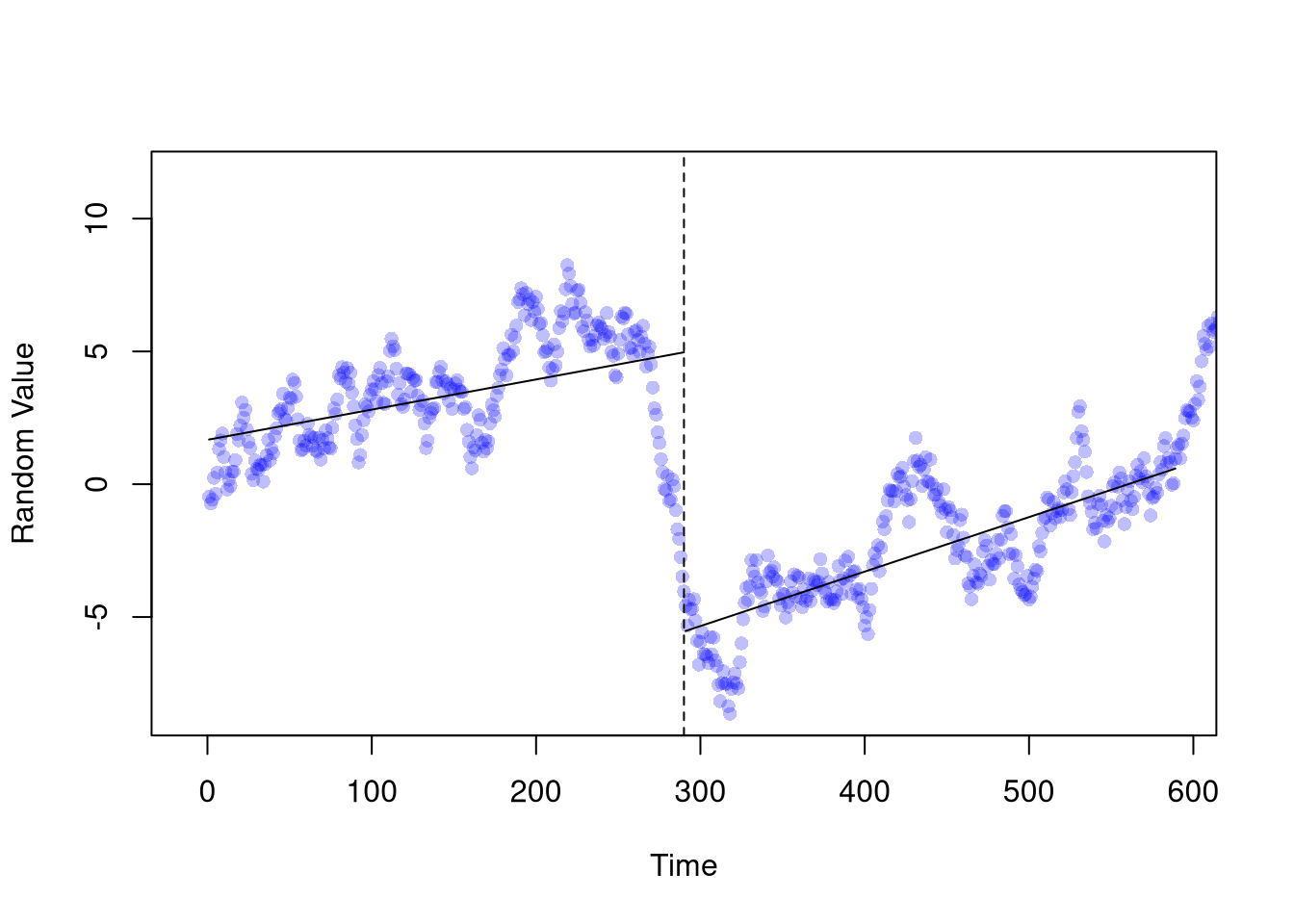
RDD. Second, find a large discrete change in the data that you can associate with a policy. You can use this as an instrument too, also providing a causal estimate of \(X_{2}\) on \(X_{1}\).
Code
# Let the data take shape
# (around the large differences before and after)
n1 <- 290
wind1 <- c(n1-300, n1+300)
dat1 <- data.frame(t=n_index, y=random_walk1, d=1*(n_index > n1))
dat1_sub <- dat1[ n_index>wind1[1] & n_index < wind1[2], ]

# Then find your big break
reg0 <- lm(y ~ t, data=dat1_sub[dat1_sub$d==0, ])
reg1 <- lm(y ~ t, data=dat1_sub[dat1_sub$d==1, ])

# The evidence should show openly (it's just science)
plot(random_walk1, pch=16, col=rgb(0, 0, 1, .25),
    xlim=wind1, xlab='Time', ylab='Random Value')
abline(v=n1, lty=2)
lines(reg0$model$t, reg0$fitted.values, col=rgb(0, 0, 0, .8))
lines(reg1$model$t, reg1$fitted.values, col=rgb(0, 0, 0, .8))
Code
# Dress with some statistics for added credibility
rdd_sub <- lm(y ~ d+t+d*t, data=dat1_sub)
rdd_full <- lm(y ~ d+t+d*t, data=dat1)
stargazer::stargazer(rdd_sub, rdd_full,
    type='html',
    title='Recipe RDD',
    header=FALSE,
    omit=c('Constant'),
    notes=c('First column uses a dataset around the discontinuity.',
    'Smaller windows are more causal, and where the effect is bigger.'))
Recipe RDD
|
|
|
|
Dependent variable:
|
|
|
|
|
|
y
|
|
|
(1)
|
(2)
|
|
|
|
d
|
-13.169***
|
-9.639***
|
|
|
(0.569)
|
(0.527)
|
|
|
|
|
|
t
|
0.011***
|
0.011***
|
|
|
(0.001)
|
(0.002)
|
|
|
|
|
|
d:t
|
0.009***
|
0.004*
|
|
|
(0.002)
|
(0.002)
|
|
|
|
|
|
|
|
Observations
|
589
|
1,000
|
|
R2
|
0.771
|
0.447
|
|
Adjusted R2
|
0.770
|
0.446
|
|
Residual Std. Error
|
1.764 (df = 585)
|
3.081 (df = 996)
|
|
F Statistic
|
658.281*** (df = 3; 585)
|
268.763*** (df = 3; 996)
|
|
|
|
Note:
|
p<0.1; p<0.05; p<0.01
|
|
|
First column uses a dataset around the discontinuity.
|
|
|
Smaller windows are more causal, and where the effect is bigger.
|
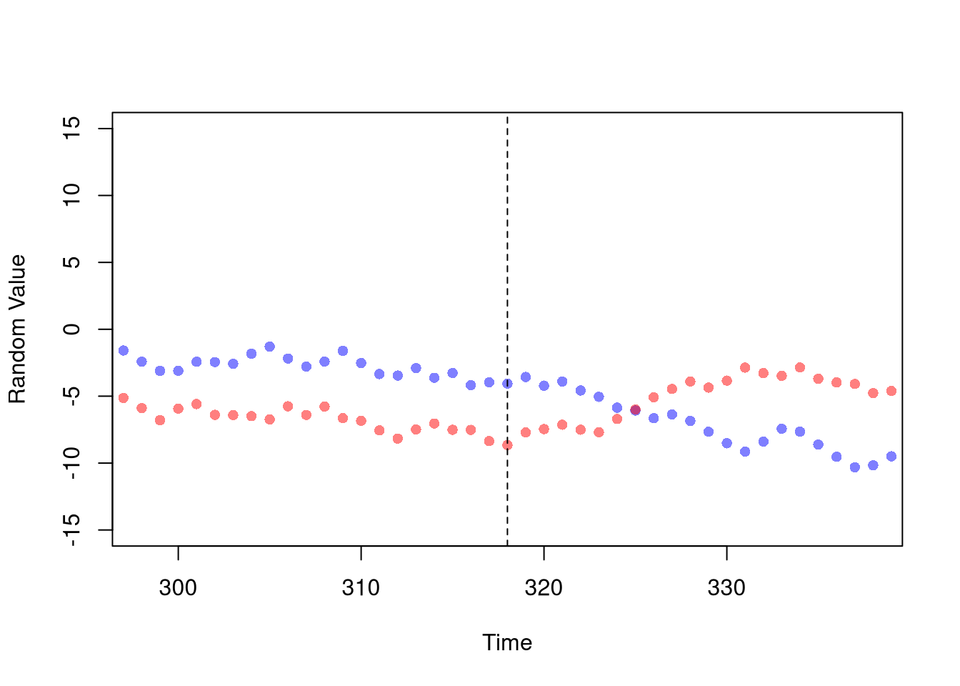
DID. Third, find a change in the data that you can associate with a policy where the control group has parallel trends. This also provides a causal estimate of \(X_{2}\) on \(X_{1}\).
Code
# Find a reversal of fortune
# (A good story always goes well with a nice pre-trend)
n2 <- 318
wind2 <- c(n2-20, n2+20)
plot(random_walk2, pch=16, col=rgb(0, 0, 1, .5),
    xlim=wind2, ylim=c(-15, 15), xlab='Time', ylab='Random Value')
points(random_walk1, pch=16, col=rgb(1, 0, 0, .5))
abline(v=n2, lty=2)
Code
# Knead out any effects that are non-causal (aka correlation)
dat2A <- data.frame(t=n_index, y=random_walk1, d=1*(n_index > n2), RWid=1)
dat2B <- data.frame(t=n_index, y=random_walk2, d=0, RWid=2)
dat2  <- rbind(dat2A, dat2B)
dat2$RWid <- as.factor(dat2$RWid)
dat2$tid <- as.factor(dat2$t)
dat2_sub <- dat2[ dat2$t>wind2[1] & dat2$t < wind2[2], ]

# Report the stars for all to enjoy
# (what about the intercept?)
# (stable coefficients are the good ones?)
did_fe1 <- lm(y ~ d+tid, data=dat2_sub)
did_fe2 <- lm(y ~ d+RWid, data=dat2_sub)
did_fe3 <- lm(y ~ d*RWid+tid, data=dat2_sub)
stargazer::stargazer(did_fe1, did_fe2, did_fe3,
    type='html',
    title='Recipe DID',
    header=FALSE,
    omit=c('tid', 'RWid', 'Constant'),
    notes=c(
     'Fixed effects for time in column 1, for id in column 2, and both in column 3.',
     'Fixed effects control for most of your concerns.',
     'Anything else creates a bias in the opposite direction.'))
Recipe DID
|
|
|
|
Dependent variable:
|
|
|
|
|
|
y
|
|
|
(1)
|
(2)
|
(3)
|
|
|
|
d
|
1.804*
|
1.847***
|
5.851***
|
|
|
(0.892)
|
(0.652)
|
(0.828)
|
|
|
|
|
|
|
|
|
Observations
|
78
|
78
|
78
|
|
R2
|
0.227
|
0.164
|
0.668
|
|
Adjusted R2
|
-0.566
|
0.142
|
0.309
|
|
Residual Std. Error
|
2.750 (df = 38)
|
2.035 (df = 75)
|
1.827 (df = 37)
|
|
F Statistic
|
0.287 (df = 39; 38)
|
7.379*** (df = 2; 75)
|
1.860** (df = 40; 37)
|
|
|
|
Note:
|
p<0.1; p<0.05; p<0.01
|
|
|
Fixed effects for time in column 1, for id in column 2, and both in column 3.
|
|
|
Fixed effects control for most of your concerns.
|
|
|
Anything else creates a bias in the opposite direction.
|
All three empirical recipes (IV, RDD, DID) produced statistically significant results from random walks with no true relationship. What is the common thread? In your own empirical work, how would you distinguish a genuine causal finding from a spurious one?
Exercises
Comment the script you wrote for this chapter, then restart R and check that it runs from a clean session, then check the script with AI as explained in Working with AI. Write three sentences from memory on the main statistical idea of this chapter, and ask the assistant what is wrong, vague, or missing. Finish with your own questions about whatever you found hardest.
Explain the difference between p-hacking and spurious regression. Both can produce statistically significant results from unrelated data, but the mechanisms differ. Give a concrete example of each using concepts from this chapter.
Using the tylervigen.csv dataset from the chapter, pick any two variables and run an OLS regression. Then pick a third variable as an instrument and run a 2SLS regression with fixest::feols. Report the p-values for both. Do these significant results reflect a real causal relationship? Why or why not?
Simulate two independent random walks of length 500 in R (each starting at 0, with increments from runif(1, -1, 1)). Regress one on the other using lm() and record the p-value on the slope. Repeat this 200 times and plot the distribution of p-values. What fraction are below 0.05, and how does this compare to what you would expect under independence?
Recall
This chapter cataloged three ways significant results arise from noise (data errors, \(p\)-hacking, and spurious regression) and showed that all three causal-inference recipes (IV, RDD, DID) can produce statistically significant findings from purely random data. The p-hacking loop made the search problem concrete: with a strict cutoff of \(p < 0.001\), the while loop kept regenerating random X2 values until it eventually hit a “significant” regression, and the cumulative-\(p\) formula \(1-(1-\alpha)^k\) showed how the chance of at least one false discovery grows past \(50\%\) by \(k=700\) tries. In the next chapter we collect the remaining multivariate topics: prediction, multiple testing corrections, and the matrix-form OLS theory that underlies everything above.
Athey, Susan, and Guido W. Imbens. 2019.
“Machine Learning Methods That Economists Should Know About.” Annual Review of Economics 11 (1): 685–725.
https://doi.org/10.1146/annurev-economics-080217-053433.