24  Experimental Data

---

The previous chapter showed how observational data complicate causal inference. This chapter introduces the standard remedies: experimental designs that combine control (the researcher fixes other factors) and randomization (the researcher manipulates one factor independently of the others), together with the quasi-experimental cousins (RDD, DID, 2SLS) that recover causal estimates when full experimental control is unavailable.

24.1 Design Basics

Control and Randomize.

What separates an experiment from an observation is the researcher’s ability to set the value of one variable and hold the others fixed.

ImportantKey Definition

Control is the researcher’s ability to hold other factors constant; randomization is the assignment of treatment in a way that is statistically independent of every pre-treatment variable.

Together control and randomization are useful because they break the correlation between a regressor and the error term that produces endogeneity in observational data. They are the only fully reliable way to estimate causal effects. You manipulate one explanatory variable while ensuring no other factors change with it, so the manipulated variable is not systematically associated with anything else.

To be concrete, we will continue with our supply and demand example from the last chapter, and this time introduce a cost shock.

Competitive Equilibrium Example.

# Demand Curve Simulator
qd_fun <- function(p, Ad=8, Bd=-.8, Ed_sigma=.25){
    Qd <- Ad + Bd*p + rnorm(1, 0, Ed_sigma)
    return(Qd)
}

# Supply Curve Simulator
qs_fun <- function(p, As=-8, Bs=1, Es_sigma=.25){
    Qs <- As + Bs*p + rnorm(1, 0, Es_sigma)
    return(Qs)
}

# Quantity Supplied and Demanded at 3 Prices
cbind(P=8:10, D=qd_fun(8:10), S=qs_fun(8:10))
##       P         D          S
## [1,]  8 1.7402575 -0.5406496
## [2,]  9 0.9402575  0.4593504
## [3,] 10 0.1402575  1.4593504

# Market Equilibrium Finder
eq_fun <- function(demand, supply, P){
    # Compute EQ (what we observe)
    eq_id <- which.min( abs(demand-supply) )
    eq <- c(P=P[eq_id], Q=demand[eq_id]) 
    return(eq)
}

N <- 300 # Number of Market Interactions
P <- seq(5, 10, by=.01) # Price Range to Consider
EQ1 <- sapply(1:N, function(n){
    # Market Data Generating Process
    demand <- qd_fun(P)
    supply <- qs_fun(P)
    eq <- eq_fun(demand, supply, P)    
    return(eq)
})
dat1 <- data.frame(t(EQ1), cost='1', T=1:N)

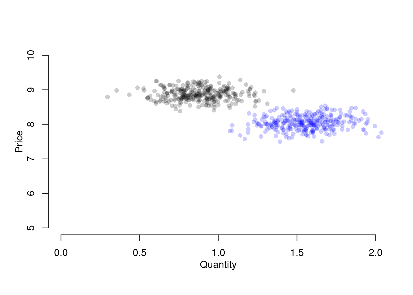
If you have exogenous variation on one side of the market, you can get information on the other. For example, lower costs shift out supply (more is produced at given price), allowing you to trace out part of a demand curve.

To see this, consider an experiment where student subjects are recruited to a classroom and randomly assigned to be either buyers or sellers in a market for little red balls. In this case, the classroom environment allows the experimenter to control for various factors (e.g., the temperature of the room is constant for all subjects) and the explicit randomization of subjects means that there are not typically systematic differences in different groups of students.

In the experiment, sellers are given linear “cost functions” that theoretically yield individual supplies like the supply equation from the previous chapter and are paid “price - cost”. Buyers are given linear “benefit functions” that theoretically yield individual demands like the demand equation from the previous chapter, and are paid “benefit - price”. The theoretical predictions are therefore given by the supply equation. Moreover, experimental manipulation of \(\alpha_{S}\) leads to \[\begin{eqnarray} \frac{d P^{*}}{d \alpha_{S}} = \frac{-1}{\beta_{D}+\beta_{S}}, \\ \frac{d Q^{*}}{d \alpha_{S}} = \frac{\beta_{D}}{\beta_{D}+\beta_{S}}. \end{eqnarray}\] In this case, the supply shock has identified the demand slope: \(-\beta_{D}=d Q^{*}/d P^{*}\).

TipTest Yourself

With the parameters in the simulation (\(\beta_D = 0.8\), \(\beta_S = 1\)), the comparative statics predict \(dP^*/d\alpha_S = -1/(0.8+1) \approx -0.56\) and \(dQ^*/d\alpha_S = 0.8/1.8 \approx 0.44\). Shifting \(\alpha_S\) from \(-8\) to \(-6.5\) (a change of \(1.5\)) predicts a price decrease of about \(0.83\) and a quantity increase of about \(0.67\).

# New Observations After Cost Change
EQ2 <- sapply(1:N, function(n){
    demand <- qd_fun(P)
    supply2 <- qs_fun(P, As=-6.5) # More Supplied at Given Price
    eq <- eq_fun(demand, supply2, P)
    return(eq)
    # lines(supply2, P, col=rgb(0, 0, 1, .01))
    #points(eq[2], eq[1], col=rgb(0, 0, 1, .05), pch=16)
})
dat2 <- data.frame(t(EQ2), cost='2', T=(1:N) + N)
dat2 <- rbind(dat1, dat2)

# Plot Simulated Market Data
cols <- ifelse(as.numeric(dat2$cost)==2, rgb(0, 0, 1, .2), rgb(0, 0, 0, .2))
plot.new()
plot.window(xlim=c(0, 2), ylim=range(P))
points(dat2$Q, dat2$P, col=cols, pch=16)
axis(1)
axis(2)
mtext('Quantity', 1, line=2)
mtext('Price', 2, line=2)

If the function forms for supply and demand are different from what we predicted, we can still measure how much the experimental manipulation of production costs affects the equilibrium quantity sold (and compare that to what was predicted).¹

24.2 Comparisons Over Time

Regression Discontinuities/Kinks.

When a treatment switches on at a known cutoff in a running variable, observations just above and just below the threshold should look identical except for the treatment.

ImportantKey Definition

A regression discontinuity design (RDD) exploits a sharp change in treatment at a known cutoff in a running variable. The treatment effect is estimated as the jump in the outcome at the cutoff. A regression kink design (RKD) exploits a change in slope rather than in level.

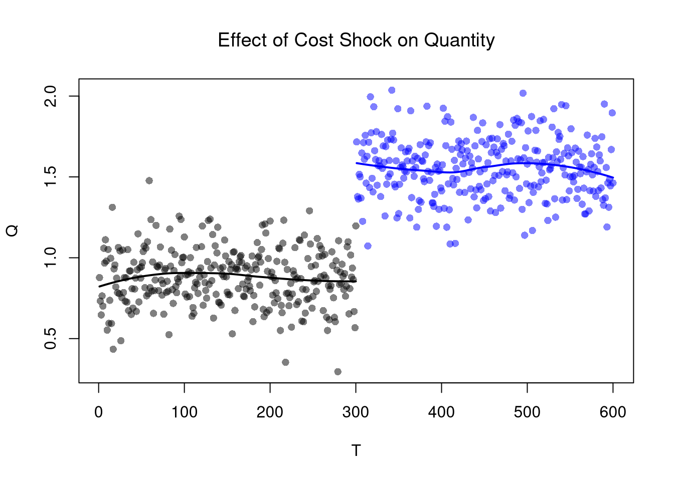
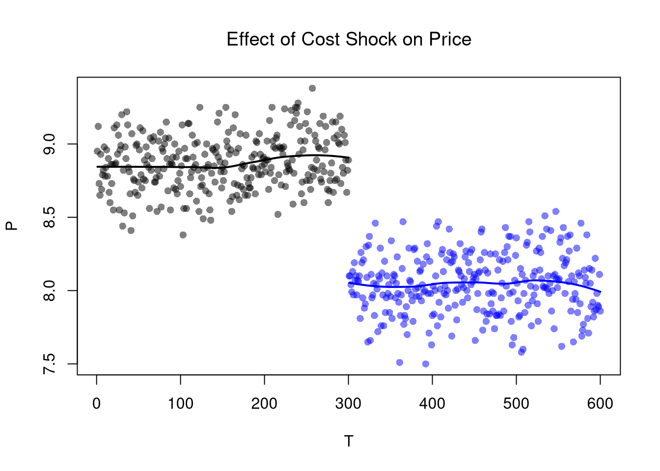
RDD/RKD is useful when a policy rule or natural threshold supplies a sharp source of exogenous variation that we can verify graphically and exploit econometrically (see The Effect, Ch. Regression Discontinuity for a thorough introduction). In our canonical competitive market example, the RDD estimate is the difference between the lines at \(T=300\).

# Locally Linear Regression 
# (Compare means near break)

cols <- ifelse(as.numeric(dat2$cost)==2, rgb(0, 0, 1, .5), rgb(0, 0, 0, .5))
plot(P ~ T, dat2, main=NA, pch=16, col=cols)
title('Effect of Cost Shock on Price', font.main=1)
regP1 <- loess(P ~ T, dat2[dat2$cost==1, ])
x1 <- regP1$x
#lm(): x1 <- regP1$model$T
lines(x1, predict(regP1), col=rgb(0, 0, 0, .8), lwd=2)
regP2 <- loess(P ~ T, dat2[dat2$cost==2, ])
x2 <- regP2$x #regP1$model$T
lines(x2, predict(regP2), col=rgb(0, 0, 1, .8), lwd=2)

plot(Q ~ T, dat2, main=NA, pch=16, col=cols)
title('Effect of Cost Shock on Quantity', font.main=1)
regQ1 <- loess(Q ~ T, dat2[dat2$cost==1, ])
lines(x1, predict(regQ1), col=rgb(0, 0, 0, .8), lwd=2)
regQ2 <- loess(Q ~ T, dat2[dat2$cost==2, ])
x2 <- regP2$x #regP1$model$T
lines(x2, predict(regQ2), col=rgb(0, 0, 1, .8), lwd=2)

# Linear Regression Alternative
sub_id <- (dat2$cost==1 & dat2$T > 250) | (dat2$cost==2 & dat2$T < 300)
dat2W <- dat2[sub_id,  ]
regP <- lm(P ~ T*cost, dat2)
regQ <- lm(Q ~ T*cost, dat2)
stargazer::stargazer(regP, regQ, 
    type='html',
    title='Recipe RDD',
    header=FALSE)

Recipe RDD

	Dependent variable:
	P	Q
	(1)	(2)
T	0.0001	-0.0001
	(0.0001)	(0.0001)
cost2	-0.875***	0.744***
	(0.066)	(0.056)
T:cost2	0.00005	-0.0001
	(0.0002)	(0.0002)
Constant	8.889***	0.911***
	(0.023)	(0.020)
Observations	600	600
R2	0.812	0.792
Adjusted R2	0.811	0.791
Residual Std. Error (df = 596)	0.202	0.172
F Statistic (df = 3; 596)	860.080***	757.320***
Note:	p<0.1; p<0.05; p<0.01

Remember that this is effect is local: different magnitudes of the cost shock or different demand curves generally yield different estimates.

NoteMust Know

The RDD estimate measures the effect at the discontinuity. Why might the effect differ for observations far from the cutoff? Give an economic example where a treatment effect varies with distance from the threshold.

Moreover, note that more than just costs have changed over time: subjects in the later periods have history experience behind them while they do not in earlier periods. So hidden variables like “beliefs” are implicitly treated as well. This is one concrete reason to have an explicit control group.

Difference in Differences.

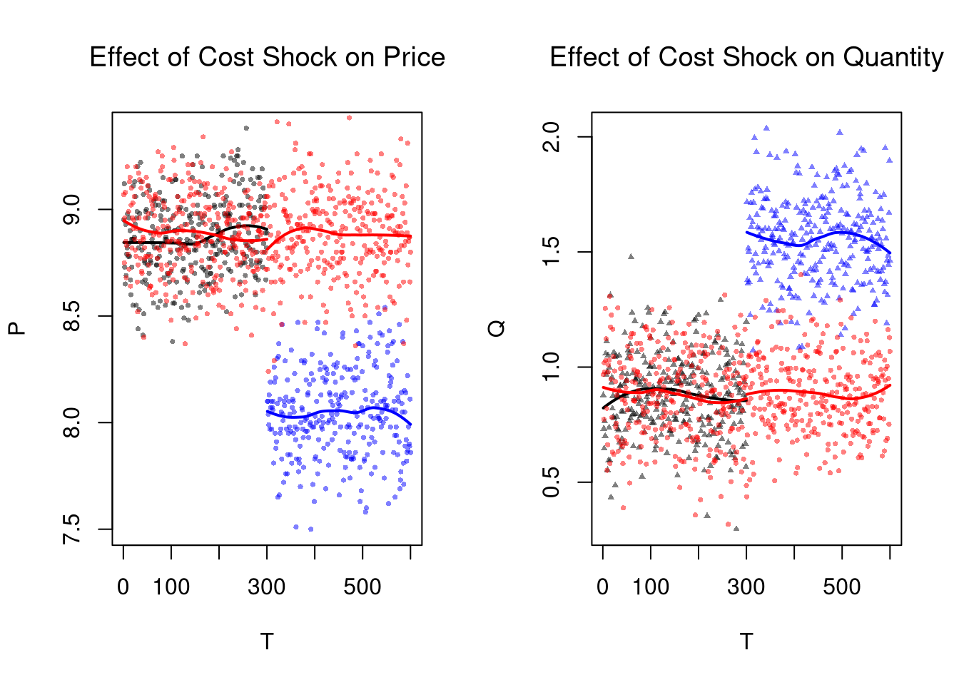
A pre/post comparison on the treated group alone confounds the treatment with anything else changing over time. We need a parallel comparison group to net it out.

ImportantKey Definition

Difference-in-differences (DID) compares the pre/post change in the outcome for a treated group to the pre/post change for a control group. The estimator is the interaction coefficient Post × Treated in a regression and relies on the parallel trends assumption: absent treatment, both groups would have followed the same trajectory.

DID is useful when a treatment hits one group but not another and we observe both before and after: the control group’s pre/post change estimates the counterfactual trend, and the treatment effect is what is left after subtracting it (see The Effect, Ch. Difference-in-Differences for more detail).

EQ3 <- sapply(1:(2*N), function(n){

    # Market Mechanisms
    demand <- qd_fun(P)
    supply <- qs_fun(P)

    # Compute EQ (what we observe)
    eq_id <- which.min( abs(demand-supply) )
    eq <- c(P=P[eq_id], Q=demand[eq_id]) 

    # Return Equilibrium Observations
    return(eq)
})
dat3 <- data.frame(t(EQ3), cost='1', T=1:ncol(EQ3))
dat3_pre  <- dat3[dat3$T <= N , ]
dat3_post <- dat3[dat3$T > N , ]

# Plot Price Data
par(mfrow=c(1, 2))
plot(P ~ T, dat2, main=NA, pch=16, col=cols, cex=.5)
title('Effect of Cost Shock on Price', font.main=1)
lines(x1, predict(regP1), col=rgb(0, 0, 0, .8), lwd=2)
lines(x2, predict(regP2), col=rgb(0, 0, 1, .8), lwd=2)
# W/ Control group
points(P ~ T, dat3, pch=16, col=rgb(1, 0, 0, .5), cex=.5)
regP3a <- loess(P ~ T, dat3_pre)
x3a <- regP3a$x
lines(x3a, predict(regP3a), col=rgb(1, 0, 0, .8), lwd=2)
regP3b <- loess(P ~ T, dat3_post)
x3b <- regP3b$x
lines(x3b, predict(regP3b), col=rgb(1, 0, 0, .8), lwd=2)


# Plot Quantity Data
plot(Q ~ T, dat2, main=NA, pch=17, col=cols, cex=.5)
title('Effect of Cost Shock on Quantity', font.main=1)
lines(x1, predict(regQ1), col=rgb(0, 0, 0, .8), lwd=2)
lines(x2, predict(regQ2), col=rgb(0, 0, 1, .8), lwd=2)
# W/ Control group
points(Q ~ T, dat3, pch=16, col=rgb(1, 0, 0, .5), cex=.5)
regQ3a <- loess(Q ~ T, dat3_pre)
lines(x3a, predict(regQ3a), col=rgb(1, 0, 0, .8), lwd=2)
regQ3b <- loess(Q ~ T, dat3_post)
lines(x3b, predict(regQ3b), col=rgb(1, 0, 0, .8), lwd=2)

Linear Regression Estimates

# Pool Data
dat_pooled <- rbind(
    cbind(dat2, EverTreated=1, PostPeriod=(dat2$T > N)),
    cbind(dat3, EverTreated=0, PostPeriod=(dat3$T > N)))
dat_pooled$EverTreated <- as.factor(dat_pooled$EverTreated)
dat_pooled$PostPeriod <- as.factor(dat_pooled$PostPeriod)

# Estimate Level Shift for Different Groups after T=300
regP <- lm(P ~ PostPeriod*EverTreated, dat_pooled)
regQ <- lm(Q ~ PostPeriod*EverTreated, dat_pooled)
stargazer::stargazer(regP, regQ, 
    type='html',
    title='Recipe DiD',
    header=FALSE)

Recipe DiD

	Dependent variable:
	P	Q
	(1)	(2)
PostPeriod	0.007	-0.002
	(0.017)	(0.014)
EverTreated1	0.005	0.009
	(0.017)	(0.014)
PostPeriodTRUE:EverTreated1	-0.844***	0.671***
	(0.024)	(0.020)
Constant	8.892***	0.894***
	(0.012)	(0.010)
Observations	1,200	1,200
R2	0.755	0.742
Adjusted R2	0.754	0.741
Residual Std. Error (df = 1196)	0.207	0.173
F Statistic (df = 3; 1196)	1,228.070***	1,144.849***
Note:	p<0.1; p<0.05; p<0.01

NoteMust Know

The DID estimate relies on the parallel trends assumption: absent treatment, the treatment and control groups would have followed the same trajectory. Look at the pre-treatment period in the plots above. Do the treated (black) and control (red) series appear to have parallel trends? What would violate this assumption?

TipTest Yourself: reading the DID table

The stargazer output for the DID model P ~ PostPeriod * EverTreated has four rows.

• The intercept is the mean of \(P\) for the control group in the pre period.
• PostPeriodTRUE is the change between pre and post in the control group.
• EverTreated1 is the pre-period difference between treated and control.
• PostPeriodTRUE:EverTreated1 is the DID estimate: the extra change in the treated group above the control trend. This is the coefficient to interpret as the treatment effect.

A statistically significant interaction term whose sign matches what theory predicts is the headline DID result. The same logic applies to the RDD table, where the T:cost2 interaction captures the change in slope at the discontinuity.

Blocking and Clustering .

When experimental units differ on a variable that also predicts the outcome, a fully random assignment can leave treatment and control unbalanced by chance.

ImportantKey Definition

Blocking partitions experimental units into homogeneous groups before randomly assigning treatment within each group.

Blocking is useful when the blocking variable predicts the outcome: it buys precision because it removes one source of between-arm variation by construction, ensuring the treatment-control comparison is balanced on the blocking variable. A fully random (“completely randomized”) design works when units are homogeneous but does not protect against accidental imbalance otherwise.

Continuing with supply and demand example, we might manipulate costs (randomize high or low treatments) for companies in different industries (computer services, lumber harvesting). With a completely randomized design, industry composition can differ between treatment and control purely by chance; blocking by industry removes that source of imbalance.

# Contrast completely randomized vs blocked assignment
set.seed(1)
industry <- rep(c('Computer', 'Lumber'), each=20)
n <- length(industry)

# Completely randomized: assign half to treatment, ignore industry
crd <- sample(rep(c('Treat','Control'), each=n/2))
table(industry, crd)
##           crd
## industry   Control Treat
##   Computer      11     9
##   Lumber         9    11

# Blocked: assign half within each industry
blocked <- character(n)
for(g in unique(industry)){
    idx <- which(industry == g)
    blocked[idx] <- sample(rep(c('Treat','Control'), each=length(idx)/2))
}
table(industry, blocked)
##           blocked
## industry   Control Treat
##   Computer      10    10
##   Lumber        10    10

Notice that the blocked design always returns 10-10 in each industry, whereas the completely randomized design can drift away from that balance from one realization to the next. Blocking buys precision when the blocking variable predicts the outcome.

24.3 Quasi Experiments

Quasi or natural experiments are historical case studies have the second distinguishing feature of experiments: randomization, but not the first: control. This helps remedy the endogeneity issues in observational data. “Instrumental Variables”, “RDD”, “DID” methods discussed above are used in historical event studies. The elementary versions use linear regression, so I can cover them here using our competitive equilibrium example from before.

Two Stage Least Squares (2SLS).

When the regressor we care about is correlated with the error term, OLS is biased. A different variable that affects the outcome only through the endogenous regressor can still recover its causal effect.

ImportantKey Definition

Two-Stage Least Squares (2SLS) uses an instrumental variable (here, the cost shock) to recover the causal effect of an endogenous regressor on an outcome. The instrument must (i) be relevant, meaning it is correlated with the endogenous regressor, and (ii) satisfy the exclusion restriction, meaning it affects the outcome only through that regressor.

2SLS is useful when controlled experimentation is impossible but a natural source of exogenous variation in the endogenous regressor is available. For example, the cost shock supplies exogenous variation in price that lets us trace out the demand curve (see The Effect, Ch. Instrumental Variables for a broader treatment). Just running a second OLS regression on the pooled data would still be biased, as we will see below.

# Not exactly right, but at least right sign
reg2 <- lm(Q ~ P, data=dat2)
summary(reg2)
## 
## Call:
## lm(formula = Q ~ P, data = dat2)
## 
## Residuals:
##      Min       1Q   Median       3Q      Max 
## -0.61599 -0.17211 -0.00927  0.16099  0.70284 
## 
## Coefficients:
##             Estimate Std. Error t value Pr(>|t|)    
## (Intercept)  6.57271    0.17682   37.17   <2e-16 ***
## P           -0.62925    0.02082  -30.22   <2e-16 ***
## ---
## Signif. codes:  0 '***' 0.001 '**' 0.01 '*' 0.05 '.' 0.1 ' ' 1
## 
## Residual standard error: 0.2369 on 598 degrees of freedom
## Multiple R-squared:  0.6043, Adjusted R-squared:  0.6036 
## F-statistic: 913.1 on 1 and 598 DF,  p-value: < 2.2e-16

It turns out that the noisiness of the process within each group affects our OLS estimate: \(\hat{B^{*}}=\hat{C}_{Q^{*}P^{*}} / \hat{V}_{P^{*}}\). For details, see

Within Group Variance

You can experiment with the effect of different variances on both OLS and IV in the code below. And note that if we had multiple supply shifts and recorded their magnitudes, then we could recover more information about demand, perhaps tracing it out entirely.

library(fixest)

# Examine
Egrid <- expand.grid(Ed_sigma=c(.001, .25, 1), Es_sigma=c(.001, .25, 1))

Egrid_regs <- lapply(1:nrow(Egrid), function(i){
    Ed_sigma <- Egrid[i, 1]
    Es_sigma <- Egrid[i, 2]
    EQ1 <- sapply(1:N, function(n){
        demand <- qd_fun(P, Ed_sigma=Ed_sigma)
        supply <- qs_fun(P, Es_sigma=Es_sigma)
        return(eq_fun(demand, supply, P))
    })
    EQ2 <- sapply(1:N, function(n){
        demand <- qd_fun(P, Ed_sigma=Ed_sigma)
        supply2 <- qs_fun(P, As=-6.5, Es_sigma=Es_sigma)
        return(eq_fun(demand, supply2, P))
    })
    dat <- rbind(
        data.frame(t(EQ1), cost='1'),
        data.frame(t(EQ2), cost='2'))
    return(dat)
})
Egrid_OLS <- sapply(Egrid_regs, function(dat) coef( lm(Q ~ P, data=dat)))
Egrid_IV <- sapply(Egrid_regs, function(dat) coef( feols(Q ~ 1|P ~ cost, data=dat)))

#cbind(Egrid, coef_OLS=t(Egrid_OLS)[, 2], coef_IV=t(Egrid_IV)[, 2])
lapply( list(Egrid_OLS, Egrid_IV), function(ei){
    Emat <- matrix(ei[2, ], 3, 3)
    rownames(Emat) <- paste0('Ed_sigma.', c(.001, .25, 1))
    colnames(Emat) <- paste0('Es_sigma.', c(.001, .25, 1))
    return( round(Emat, 2))
})
## [[1]]
##                Es_sigma.0.001 Es_sigma.0.25 Es_sigma.1
## Ed_sigma.0.001           -0.8         -0.80      -0.80
## Ed_sigma.0.25            -0.6         -0.64      -0.71
## Ed_sigma.1                0.3          0.28      -0.05
## 
## [[2]]
##                Es_sigma.0.001 Es_sigma.0.25 Es_sigma.1
## Ed_sigma.0.001          -0.80         -0.80      -0.80
## Ed_sigma.0.25           -0.80         -0.80      -0.84
## Ed_sigma.1              -0.68         -0.78      -0.79

To overcome this issue, we can compute the change in the expected values \(d \mathbb{E}[Q^{*}] / d \mathbb{E}[P^{*}] =-\beta_{D}\). Empirically, this is estimated via the change in average value.

# Wald (1940) Estimate
dat_mean <- rbind(
    colMeans(dat2[dat2$cost==1, 1:2]),
    colMeans(dat2[dat2$cost==2, 1:2]))
dat_mean
##           P         Q
## [1,] 8.8971 0.9031814
## [2,] 8.0601 1.5719325
B_est <- diff(dat_mean[, 2])/diff(dat_mean[, 1])
round(B_est, 2)
## [1] -0.8

We can also separately recover \(d \mathbb{E}[Q^{*}] / d \mathbb{E}[\alpha_{S}]\) and \(d \mathbb{E}[P^{*}] / d \mathbb{E}[\alpha_{S}]\) from separate regressions.²

# Heckman (2000, p.58) Estimate
ols_1 <- lm(P ~ cost, data=dat2)
ols_2 <- lm(Q ~ cost, data=dat2)
B_est2 <- coef(ols_2)/coef(ols_1)
round(B_est2[[2]], 2)
## [1] -0.8

Alternatively, we can recover the same estimate using a 2SLS regression with two equations: \[\begin{eqnarray} \hat{P} &=& b_{0p} + b_{1p} \alpha_{S} + e_{p} \\ \hat{Q} &=& b_{0q} + b_{1q} \hat{p} + e_{q}. \end{eqnarray}\] where \(\hat{p}\), the predicted value of \(\hat{P}\) from the first equation, is used to explain quantity in the second equation. In the first regression, we estimate how the cost shock affects prices: \(\hat{b}_{1p}\) and then predict prices \(\hat{p}\). In the second equation, we estimate how the average effect of predicted prices (which are exogenous to demand) affect quantity demanded.

To understand this theoretically, first substitute the equilibrium condition into the supply equation: \(Q_{D}=Q_{S}=\alpha_{S}+ \beta_{S} P + E_{S}\), lets us rewrite \(P\) as a function of \(Q_{D}\). This yields two theoretical equations. We are using the cost shock to understand the theoretical demand curve. \[\begin{eqnarray} P &=& -\frac{\alpha_{S}}{{\beta_{S}}} + \frac{Q_{D}}{\beta_{S}} - \frac{E_{S}}{\beta_{S}} \\ Q_{D} &=& \alpha_{D} + \beta_{D} P + E_{D}. \end{eqnarray}\]

# Two Stage Least Squares Estimate
ols_1 <- lm(P ~ cost, data=dat2)
dat2_new  <- cbind(dat2, Phat=predict(ols_1))
reg_2sls <- lm(Q ~ Phat, data=dat2_new)
summary(reg_2sls)
## 
## Call:
## lm(formula = Q ~ Phat, data = dat2_new)
## 
## Residuals:
##     Min      1Q  Median      3Q     Max 
## -0.5517 -0.1177 -0.0055  0.1185  0.5254 
## 
## Coefficients:
##             Estimate Std. Error t value Pr(>|t|)    
## (Intercept)  8.01184    0.14248   56.23   <2e-16 ***
## Phat        -0.79899    0.01678  -47.60   <2e-16 ***
## ---
## Signif. codes:  0 '***' 0.001 '**' 0.01 '*' 0.05 '.' 0.1 ' ' 1
## 
## Residual standard error: 0.1721 on 598 degrees of freedom
## Multiple R-squared:  0.7912, Adjusted R-squared:  0.7909 
## F-statistic:  2266 on 1 and 598 DF,  p-value: < 2.2e-16

# One Stage Instrumental Variables Estimate
library(fixest)
reg2_iv <- feols(Q ~ 1|P ~ cost, data=dat2)
summary(reg2_iv)
## TSLS estimation: Second stage
## |- D.V.   : Q
## |- Endo.  : P
## |- Instr. : cost
## Dep. Var.: Q
## Observations: 600
## Standard-errors: IID 
##              Estimate Std. Error  t value  Pr(>|t|)    
## (Intercept)  8.011838   0.206765  38.7486 < 2.2e-16 ***
## fit_P       -0.798986   0.024357 -32.8031 < 2.2e-16 ***
## ---
## Signif. codes:  0 '***' 0.001 '**' 0.01 '*' 0.05 '.' 0.1 ' ' 1
## RMSE: 0.24927   Adj. R2: 0.790851
## F-test (1st stage), P: stat = 2,585.06, p < 2.2e-16, on 1 and 598 DoF.
##            Wu-Hausman: stat =   551.70, p < 2.2e-16, on 1 and 597 DoF.

The Wald, Heckman, and 2SLS slopes are algebraically identical in this just-identified linear model: each one recovers \(-\beta_{D}\) by using the cost shock as the source of exogenous variation in price.

TipTest Yourself

The 2SLS procedure works in two steps. First, regress the endogenous variable (price) on the instrument (cost): this isolates the part of price variation driven by supply shifts. Second, regress quantity on the predicted prices from step 1. Because predicted prices reflect only supply-side variation, the second-stage coefficient estimates the demand slope. The key requirement is that cost shifts affect quantity only through price (the exclusion restriction).

Caveats.

2SLS regression analysis can be very insightful, but I also want to stress some caveats about their practical application. Most of which stem directly from the absence of control that true experiments have.

• Instrument exogeneity (Exclusion Restriction): The instrument must affect outcomes only through the treatment variable (e.g., only supply is affected directly, not demand).
• Instrument relevance: The instrument must be strongly correlated with the endogenous regressor, implying the shock creates meaningful variation.
• Functional form correctness: Supply and demand are assumed linear and additively separable.
• Multiple hypothesis testing risks: We were not repeatedly testing different instruments, which can artificially produce significant findings by chance.
• Exclusion restriction violations: Spatial or temporal spillovers may cause instruments to affect the outcome through unintended channels, undermining instrument exogeneity.
• Weak instruments: Spatial clustering, serial correlation, or network interdependencies can reduce instrument variation, causing weak instruments.
• Inference and standard errors: Spatial or temporal interdependence reduces the effective sample size, making conventional standard errors misleadingly small.

We always get coefficients back when running feols, and sometimes the computed p-values are very small. The interpretation of those numbers rests on many assumptions, and we are rarely sure that all of these assumptions hold. Researchers often also report their OLS results, but that is insufficient. A nonparametric estimator (e.g. loess) at each stage can help diagnose departures from linearity; other packages such as ivreg::ivreg provide alternative IV implementations. The next chapter pushes this caution further, showing that the same recipes can produce statistically significant results from data with no causal structure at all.

24.4 Exercises

1. Comment the script you wrote for this chapter, then restart R and check that it runs from a clean session, then check the script with AI as explained in Working with AI. Write three sentences from memory on the main statistical idea of this chapter, and ask the assistant what is wrong, vague, or missing. Finish with your own questions about whatever you found hardest.

2. In the competitive market simulation, a supply cost shock is used to identify the demand slope via 2SLS. Explain why simply regressing \(Q\) on \(P\) with both cost regimes pooled does not recover the demand slope \(-\beta_D\), and what role the exclusion restriction plays in the 2SLS approach.

3. Using the pooled market data (dat2) from the chapter, compute the Wald estimate of the demand slope by hand: take the difference in mean quantity across cost groups divided by the difference in mean price. Compare this to the 2SLS estimate from fixest::feols(Q ~ 1 | P ~ cost, data = dat2). Are they the same? Why or why not?

4. Simulate a difference-in-differences setup in R. Generate two groups of 100 observations each over 200 time periods, where one group receives a treatment (a level shift of +2) at \(T = 100\). Estimate the DID coefficient using lm(y ~ PostPeriod * EverTreated, data = dat) and verify that it recovers the treatment effect.

Further Reading.

The following resources discuss causal inference methods (IV, RDD, DID) in more detail.

• https://mixtape.scunning.com/ – Cunningham’s Causal Inference: The Mixtape, a free online textbook covering IV, RDD, DID, and synthetic control with code examples.
• https://theeffectbook.net/ – Huntington-Klein’s The Effect, an accessible introduction to research design and causal identification.
• https://www.econometrics-with-r.org/12-ivr.html – instrumental variables regression in R with practical worked examples.

Recall

This chapter introduced the experimental and quasi-experimental tools for recovering causal effects from data with limited control: RDD, DID, blocking, and 2SLS. The cost-shock experiment threaded through the chapter made the trade-off explicit: with \(\alpha_S = -8\) vs \(-6.5\) in qs_fun, the Wald, Heckman, and 2SLS estimates of \(-\beta_D\) from feols(Q ~ 1 | P ~ cost, data=dat2) are algebraically identical and recover the demand slope that pooled OLS confused. In the next chapter we caution that the same recipes can produce statistically significant findings from data that contain no causal signal at all.

---

1. Notice that even in this linear model, however, all effects are conditional: The effect of a cost change on quantity or price depends on the demand curve. A change in costs affects quantity supplied but not quantity demanded (which then affects equilibrium price) but the demand side of the market still matters! The change in price from a change in costs depends on the elasticity of demand.

2. Mathematically, we can also do this in a single step by exploiting linear algebra: \(\frac{\frac{ Cov(Q^{*},\alpha_{S})}{ V(\alpha_{S}) } }{\frac{ Cov(P^{*},\alpha_{S})}{ V(\alpha_{S}) }} = \frac{Cov(Q^{*},\alpha_{S} )}{ Cov(P^{*},\alpha_{S})}.\)