We will now dig a little deeper theoretically into the statistics we compute. When we know how the data are generated theoretically, we can often compute the theoretical value of the two most basic and often-used statistics: the mean and variance.
This chapter asks three questions.
- What does a statistic estimate?
- Parameter, estimator, and estimate: these separate a fixed population number, a formula for any sample, and the specific number from our sample.
- Expected value and population variance: these are the theoretical mean and variance, computed from known probabilities.
- Plug-in principle: this puts sample proportions into a population formula, which recovers the sample mean and variance.
- How sure are we?
- Mean and variance of the sample mean: these are \(\mathbb{E}[M]=\mathbb{E}[X_{i}]\), from linearity of expectation, and \(\mathbb{V}[M]=\mathbb{V}[X_{i}]/n\), which shrinks like \(1/n\). These two results set the center and spread of the Normal curve in the central limit theorem, but they do not explain why the curve is Normal.
- Standard error formula: this estimates \(\text{SE}(M)\) with \(\hat{s}/\sqrt{n}\), as an alternative to the bootstrap.
- Law of the Unconscious Statistician (LOTUS): this gives the expected value of a function of \(X_{i}\) without first deriving that function’s distribution. It supplies the center and spread of the Normal curve for the variance estimator \(V\).
- How do we judge an estimator?
- Bias: this asks whether an estimator is right on average. The divide-by-\(n\) variance estimator is biased, so we often use the adjusted sample standard deviation \(\hat{s}_{\text{adj}}\), which divides by \(n-1\).
- Consistency: this asks whether estimates get closer to the parameter as the sample grows. The shrinking variance explains why the sample mean is consistent, which is the law of large numbers.
Statistical Theory
Recall that we denote \(X_{i}\) as a random variable that can take on specific values \(x\) from the sample space with known probabilities (see this probability refresher if needed). For example, \(X_{i}\) is a coin that we will flip and it can land on heads (\(x=1\)) or tails (\(x=0\)).
- \(X_{i}\) is a random variable, taking on outcomes \(x\)
- \(\hat{x}_{i}\) is a realized value
Three related terms are easy to mix up.
A population parameter is a fixed but typically unknown number describing the population distribution.
An estimator is a random variable: a formula that computes a statistic on any sample of size \(n\) from the population.
An estimate is the specific number you get by applying the estimator to your particular sample.
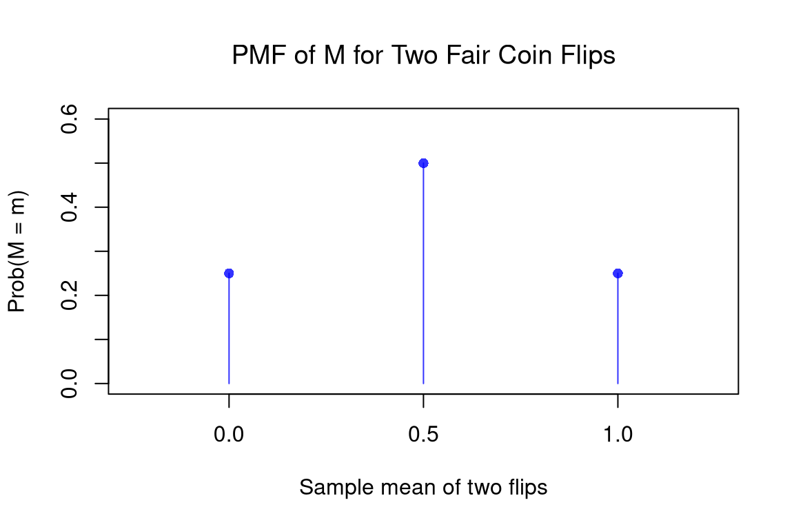
The distinction is useful for being precise about uncertainty. A parameter is just an unknown number, so it has no sampling variability. An estimator has a full sampling distribution, and an estimate is one realization from that distribution. For example, consider flipping a fair coin twice. The estimator \(M = (X_{1}+X_{2})/2\) is computed on coins before they are flipped. There are four possible samples, HH, HT, TH, and TT, each with probability \(1/4\). Computing \(M\) in each sample gives \[\begin{aligned}
\text{HH}: \quad M &= (1+1)/2 = 1 \\
\text{HT}: \quad M &= (1+0)/2 = 1/2 \\
\text{TH}: \quad M &= (0+1)/2 = 1/2 \\
\text{TT}: \quad M &= (0+0)/2 = 0.
\end{aligned}\] So the PMF of \(M\) is \(\text{Prob}(M=0)=1/4\), \(\text{Prob}(M=1/2)=1/4+1/4=1/2\), and \(\text{Prob}(M=1)=1/4\). This PMF is the sampling distribution of \(M\).
Code
## MAIN EXAMPLE
# M in each of the four samples HH, HT, TH, TT
x1 <- c(1, 1, 0, 0) # first flip
x2 <- c(1, 0, 1, 0) # second flip
m_samples <- (x1 + x2)/2
m_samples
## [1] 1.0 0.5 0.5 0.0

# PMF of M, since each sample has probability 1/4
m_probs <- c(table(m_samples))/4
m_values <- as.numeric(names(m_probs))
m_probs
##    0  0.5    1
## 0.25 0.50 0.25

plot(m_values, m_probs, type='h', col=rgb(0, 0, 1, .8),
    xlim=c(-0.25, 1.25), ylim=c(0, 0.6),
    main=NA, xlab='Sample mean of two flips', ylab='Prob(M = m)')
points(m_values, m_probs, pch=16, col=rgb(0, 0, 1, .8))
title('PMF of M for Two Fair Coin Flips', font.main=1)
The estimate \(\hat{m}\) is the specific value after you flip them, such as \(\hat{m}=1\) if both land heads. The parameter \(\mathbb{E}[X_{i}]\) is the theoretical value \(\frac{1}{2}0 + \frac{1}{2}1=1/2\).
Random Variables used parameter for the numbers that pin down a distribution, such as the Bernoulli success probability \(\theta\) or the Exponential rate \(\lambda\). Numbers computed from these distribution parameters are also parameters, such as the Exponential mean \(\mathbb{E}[X_{i}]=1/\lambda\). For the fair coin, the two coincide: \(\theta=\mathbb{E}[X_{i}]=1/2\).
Statistical definitions
| Estimate |
\(\hat{m}\), \(\hat{v}\) |
one number you compute for a single sample of size \(n\) |
empirical mean, variance |
sample mean, uncorrected sample variance (divide-by-\(n\)) |
| Estimator |
\(M\), \(V\) |
a random variable, formula that computes the statistic for any sample of size \(n\) |
|
|
| Population |
\(\mathbb{E}[X_{i}]\), \(\mathbb{V}[X_{i}]\) |
a number defined by the theoretical distribution |
theoretical mean, variance |
population/long-run mean, variance |
For example, pretend the data are the whole population, as in Sampling & Resampling. Their average is a parameter. The sample mean formula, applied to any sample of \(n\) observations, is an estimator. The number it returns for one particular sample of \(n\) observations is an estimate.
For concreteness, we separately analyze how the theoretical mean and variance are computed for discrete and continuous random variables.
Population Parameters
Expected Value and Variance
When we know the theoretical probabilities, the two most basic summaries (center and spread) can be computed exactly rather than estimated.
The expected value (or population mean) of a random variable \(X_{i}\), written \(\mathbb{E}[X_{i}]\), is the probability-weighted average of its values. The population variance, written \(\mathbb{V}[X_{i}]\), is the expected squared deviation from \(\mathbb{E}[X_{i}]\).
These population quantities are useful as targets. Estimators from earlier chapters, like the sample mean, try to recover them. Sampling theory studies how far an estimator can fall from its target. The subsections below show how to compute these for discrete and continuous random variables.
Discrete Random Variables
If the sample space is discrete, we can compute the expected value, or theoretical mean, as \[
\mathbb{E}[X_{i}] = \sum_{x} x \text{Prob}(X_{i}=x),
\] where \(\mathbb{E}\) is the expectation function that explicitly uses the population distribution via \(\text{Prob}(X_{i}=x)\): the probability the random variable \(X_{i}\) takes the particular value \(x\). Similarly, we can compute the population variance as \[
\mathbb{V}[X_{i}] = \mathbb{E}[(X_{i}-\mathbb{E}[X_{i}])^2] = \sum_{x} \left(x - \mathbb{E}[X_{i}] \right)^2 \text{Prob}(X_{i}=x),
\] where \(\mathbb{V}\) is the variance function which also explicitly uses the population distribution. The population standard deviation is \(\sqrt{\mathbb{V}[X_{i}]}\), which measures the spread of the distribution of individual outcomes around the theoretical mean.
For example, consider a five-sided die with equal probability of landing on each side. I.e., \(X_{i}\) is a Discrete Uniform random variable with outcomes \(x~\text{in}~\{1,2,3,4,5\}\). What is the theoretical mean? What is the variance and standard deviation? \[\begin{aligned}
\mathbb{E}[X_{i}] &= 1\frac{1}{5} + 2\frac{1}{5} + 3\frac{1}{5} + 4\frac{1}{5} + 5\frac{1}{5} = 15/5 = 3 \\
\mathbb{V}[X_{i}] &= (1-3)^2\frac{1}{5} +
(2 - 3)^2\frac{1}{5} +
(3 - 3)^2\frac{1}{5} +
(4 - 3)^2\frac{1}{5} +
(5 - 3)^2\frac{1}{5} \\
&= 2^2 \frac{1}{5} + 1^2\frac{1}{5} + 0^2 \frac{1}{5} + 1^2\frac{1}{5} + 2^2 \frac{1}{5}
= (4 + 1 + 1 + 4)/5 = 10/5 = 2 \\
\sqrt{\mathbb{V}[X_{i}]} &= \sqrt{2}
\end{aligned}\]
Code
# Computerized Way to Compute Mean
x <- c(1, 2, 3, 4, 5)
x_probs <- c(1/5, 1/5, 1/5, 1/5, 1/5)
population_mean <- sum(x*x_probs)
population_mean
## [1] 3

# Computerized Way to Compute SD
population_var <- sum((x-population_mean)^2*x_probs)
population_var
## [1] 2
population_sd <- sqrt(population_var)
population_sd
## [1] 1.414214

# Verified by simulation
x_sim_hat <- sample(x, prob=x_probs,
          size=10000, replace=TRUE)
mean(x_sim_hat)
## [1] 2.9651
sqrt(mean((x_sim_hat - mean(x_sim_hat))^2)) # divides by n, unlike sd()
## [1] 1.409497
A finite population is also a discrete random variable. In Sampling & Resampling, we pretended the data were the whole population. Drawing one observation at random gives each of the \(N\) observations a probability of \(1/N\), so the population mean and variance follow directly from the formulas above.
Code
## MAIN EXAMPLE
# Pretend the 3294 workers in Wages1 are the whole population
data(Wages1, package='Ecdat')
population_wages <- Wages1[, 'wage'] # hourly wage in 1980 dollars
N <- length(population_wages)
wage_probs <- rep(1/N, N) # each worker equally likely, with probability 1/3294

# Population mean and variance, from the formulas
population_wage_mean <- sum(population_wages * wage_probs)
population_wage_mean
## [1] 5.757585
population_wage_var <- sum((population_wages - population_wage_mean)^2 * wage_probs)
population_wage_var
## [1] 10.68433
sqrt(population_wage_var) ##sd
## [1] 3.26869
With equal probabilities, \(\mathbb{E}[X_{i}]\) is just the average over the whole population, which mean() computes. Note that var() would divide by \(N-1\) instead of \(N\), and so differs slightly from \(\mathbb{V}[X_{i}]\) when \(N\) is large.
For example, an unfair coin with a \(3/4\) probability of heads (\(x=1\)) and a \(1/4\) probability of tails (\(x=0\)) has a theoretical mean of \[
\mathbb{E}[X_{i}] = 0\frac{1}{4} + 1\frac{3}{4} = \frac{3}{4}
\] and a theoretical variance of \[
\mathbb{V}[X_{i}] = [0 - \frac{3}{4}]^2 \frac{1}{4} + [1 - \frac{3}{4}]^2 \frac{3}{4}
= \frac{9}{64} + \frac{3}{64}
= \frac{12}{64}
= \frac{3}{16}.
\] Verify both the mean and variance by simulation.
Code
# A simulation of many coin flips
x <- c(0, 1)
x_probs <- c(1/4, 3/4)
x_sim <- sample(x, prob=x_probs, size=1000, replace=TRUE)

round( mean(x_sim), 4)
## [1] 0.737

round( mean((x_sim - mean(x_sim))^2), 4)
## [1] 0.1938
Consider a four-sided die with outcomes \(\{1,2,3,4\}\) and corresponding probabilities \(\{1/8, 2/8, 1/8, 4/8\}\). The mean is \[
\mathbb{E}[X_{i}] = 1 \frac{1}{8} + 2 \frac{2}{8} + 3 \frac{1}{8} + 4 \frac{4}{8} = 3.
\] The variance is the probability-weighted average squared deviation from the mean, \[
\mathbb{V}[X_{i}] = (1-3)^2 \frac{1}{8} + (2-3)^2 \frac{2}{8} + (3-3)^2 \frac{1}{8} + (4-3)^2 \frac{4}{8} = \frac{4 + 2 + 0 + 4}{8} = \frac{10}{8} = 1.25.
\]
Code
x <- c(1, 2, 3, 4)
x_probs <- c(1/8, 2/8, 1/8, 4/8)
population_mean <- sum(x * x_probs)
population_mean
## [1] 3

population_var <- sum((x - population_mean)^2 * x_probs)
population_var
## [1] 1.25

# Verify by simulation
x_sim <- sample(x, prob=x_probs, size=10000, replace=TRUE)
round(mean(x_sim), 2)
## [1] 3
round(mean((x_sim - mean(x_sim))^2), 2)
## [1] 1.25
Consider an unfair coin with a \(\theta\) probability of heads (\(x=1\)) and a \(1-\theta\) probability of tails (\(x=0\)), where \(\theta\) is a distribution parameter between \(0\) and \(1\). The theoretical mean is \[
\mathbb{E}[X_{i}] = 1[\theta] + 0[1-\theta] = \theta
\] and the theoretical variance is \[
\mathbb{V}[X_{i}]
= [1 - \theta]^2 \theta + [0 - \theta]^2 [1-\theta] = [1 - \theta]^2 \theta + \theta^2 [1-\theta]
= [1-\theta]\theta\left( [1-\theta] + \theta\right) = [1-\theta] \theta.
\] So the theoretical standard deviation is \(\sqrt{\mathbb{V}[X_{i}]}=\sqrt{[1-\theta] \theta}\).
Suppose \(X_{i}\) is a discrete random variable with this probability mass function: \[\begin{aligned}
X_{i} &= \begin{cases}
-1 & \text{ with probability } \frac{1}{2 \lambda^2} \\
0 & \text{ with probability } 1-\frac{1}{\lambda^2} \\
+1 & \text{ with probability } \frac{1}{2\lambda^2}
\end{cases},
\end{aligned}\] where \(\lambda \geq 1\) is a distribution parameter. What is the theoretical standard deviation?
For a discrete uniform random variable with the sample space \(\{1,2,3,4,5\}\), calculate the theoretical median and IQR.
Continuous Random Variables
The distribution parameters of a continuous random variable determine its mean and variance. For example, an exponential random variable with rate parameter \(\lambda\) has theoretical mean \(\mathbb{E}[X_{i}]=1/\lambda\) and variance \(\mathbb{V}[X_{i}]=1/\lambda^2\). For a normal random variable, we can specify its theoretical mean \(\mathbb{E}[X_{i}]=\mu\) and variance \(\mathbb{V}[X_{i}]=\sigma^2\) directly.
An exponential random variable with \(\lambda=2\) has \(\mathbb{E}[X_{i}]=1/2\). R’s rnorm() takes the mean and standard deviation, so the normal draws below have \(\mathbb{E}[X_{i}]=1\) and \(\mathbb{V}[X_{i}]=2^2=4\).
Code
# Exponential Random Variable
x_sim <- rexp(5000, 2)
m_hat <- mean(x_sim)
round(m_hat, 2)
## [1] 0.5

# Normal Random Variable
x_sim <- rnorm(5000, 1, 2)
round(mean(x_sim), 2)
## [1] 1.02
round(mean((x_sim - mean(x_sim))^2), 2)
## [1] 3.98
Data recorded to many decimal places can also be treated as continuous, with a density \(f(x)\) that a histogram approximates. The integral \(\mathbb{E}[X_{i}]=\int x f(x) dx\) is then approximated by a sum over the histogram bins: each bin midpoint times the area of its bar.
Code
# Wages are recorded to many decimal places, so treat them as continuous.
f_hat <- hist(population_wages, breaks=seq(0, 40, by=1), plot=FALSE)
bin_areas <- f_hat[['density']] * diff(f_hat[['breaks']]) # f(x) dx

# Mean from the histogram, and the exact population mean
sum(f_hat[['mids']] * bin_areas)
## [1] 5.757134
population_wage_mean
## [1] 5.757585
# The two numbers are close, 5.757 and 5.758.
As the bins get narrower, the sum approaches the exact mean.
If the sample space is continuous, we can compute the theoretical mean (or expected value) as \[
\mathbb{E}[X_{i}] = \int x f(x) d x,
\] where \(f(x)\) is the probability density for the particular value \(x\). Note that this is not a probability; probabilities are areas under \(f\).
Similarly, we can compute the theoretical variance as \[
\mathbb{V}[X_{i}]= \int \left(x - \mathbb{E}[X_{i}] \right)^2 f(x) d x.
\]
For example, consider a random variable with a continuous uniform distribution over \([-1, 1]\). In this case, \(f(x)=1/[1 - (-1)]=1/2\) for each \(x~\text{in}~[-1, 1]\) and \[
\mathbb{E}[X_{i}] = \int_{-1}^{1} \frac{x}{2} d x = \int_{-1}^{0} \frac{x}{2} d x + \int_{0}^{1} \frac{x}{2} d x = 0
\] and \[
\mathbb{V}[X_{i}]= \int_{-1}^{1} x^2 \frac{1}{2} d x = \frac{1}{2} \frac{x^3}{3}|_{-1}^{1} = \frac{1}{6}[1 - (-1)] = 2/6 =1/3
\]
Code
# Verify by simulation
x_sim <- runif(100000, -1, 1)
round( mean(x_sim), 2)
## [1] 0
round( mean((x_sim - mean(x_sim))^2), 2)
## [1] 0.33
Estimates
Each population formula above has a sample counterpart. Replace \(\text{Prob}(X_{i}=x)\) with the sample proportion \(\hat{p}(x)\) from the empirical mass function. The expected value and variance then become the sample mean and the divide-by-\(n\) sample variance from Summary Statistics, \[\begin{aligned}
\hat{m} &= \sum_{x} x \hat{p}(x) \\
\hat{v} &= \sum_{x} \left(x - \hat{m}\right)^2 \hat{p}(x).
\end{aligned}\] Building an estimate this way, by putting sample proportions into a population formula, is called the plug-in principle. The same substitution works for other parameters.
Suppose we flipped a coin \(100\) times and found that \(75\) were heads and \(25\) were tails. The estimated probabilities are \(\hat{p}(1)=75/100=3/4\) and \(\hat{p}(0)=25/100=1/4\), so \[\begin{aligned}
\hat{m} &= 1 \times \frac{3}{4} + 0 \times \frac{1}{4} = \frac{3}{4} \\
\hat{v} &= \left(1-\frac{3}{4}\right)^2 \times \frac{3}{4} + \left(0-\frac{3}{4}\right)^2 \times \frac{1}{4} = \frac{3}{64} + \frac{9}{64} = \frac{12}{64} = \frac{3}{16}.
\end{aligned}\] These are the plug-in versions of the theoretical coin mean \(\theta\) and variance \([1-\theta]\theta\), with \(\hat{m}\) in place of \(\theta\): \(\hat{m}(1-\hat{m}) = 3/4 \times 1/4 = 3/16\).
Code
x0_hat <- c(rep(1, 75), rep(0, 25)) # 75 heads and 25 tails
p_hat <- table(x0_hat)/length(x0_hat)
x <- as.numeric(names(p_hat))
m_hat <- sum(x * p_hat)
v_hat <- sum((x - m_hat)^2 * p_hat)
c(m_hat, v_hat)
## [1] 0.7500 0.1875
With many unique values, the plug-in mean and variance still match the averages over the observations. To see this, take one sample from the pretend population, as if it were all we observed.
Code
## MAIN EXAMPLE
# One sample of 50 workers, as if it were all we observed
x_sim <- sample(population_wages, 50, replace=FALSE)

# Wages have many unique values.
# Plug-in mean and variance, from the estimated probability of each unique value
p_hat <- table(x_sim)/length(x_sim)
x <- as.numeric(names(p_hat))
m_hat <- sum(x * p_hat)
v_hat <- sum((x - m_hat)^2 * p_hat)
round(c(m_hat, v_hat), 4)
## [1]  6.1480 12.7499

# Same numbers, from the observations directly
round(c(mean(x_sim), mean((x_sim - mean(x_sim))^2)), 4)
## [1]  6.1480 12.7499

# Population parameters, which these numbers estimate
round(c(population_wage_mean, population_wage_var), 4)
## [1]  5.7576 10.6843
# The estimates, about 6.15 and 12.75, differ from these parameters.
An estimate can differ from its population parameter because it comes from only one sample.
You can estimate means and variances for continuous random variables with weights, but here we have an additional approximation error due to binning by the histogram.
Code
x_sim <- rnorm(5000, 1, 2) # continuous draws, as in Continuous Random Variables

# values and probabilities
f_hat  <- hist(x_sim, plot=FALSE)
wt <- f_hat[['counts']]/length(x_sim)
xt <- f_hat[['mids']]
# Weighted mean
m_hat <- sum(wt*xt)
m_hat
## [1] 0.9946

# Compare to 'mean(x_sim)'
Try it yourself with
Code
x_sim <- runif(2000, -1, 1)
Estimators
Means
The LLN says the sample mean concentrates on the population mean as \(n\) grows. To explain it, we first find where the sampling distribution of \(M\) is centered, using a basic rule about how expectations distribute over sums. Linearity of expectation states that for any random variables \(X_{1}, X_{2}\) and constants \(a, b\), \[\mathbb{E}[a X_{1} + b X_{2}] = a \mathbb{E}[X_{1}] + b \mathbb{E}[X_{2}].\] This is useful because it lets us reason about the mean of any linear combination of random variables without computing a joint distribution.
Applied to the sample mean estimator \(M = \sum_{i=1}^{n} X_{i}/n\), with the constants \(1/n\): \[
\mathbb{E}\left[M\right] = \mathbb{E}\left[ \sum_{i=1}^{n} X_{i}/n \right] = \sum_{i=1}^{n} \mathbb{E}[X_{i}]/n.
\] Assuming each observation has the same finite expected value, the expected value of the sample average equals this common population mean: \(\mathbb{E}\left[M\right] = \mathbb{E}[X_{i}]\) for every \(i\). For a detailed treatment, see here.
Return to the two fair coin flips in Statistical Theory, where \(\mathbb{E}[X_{1}]=\mathbb{E}[X_{2}]=1/2\) and each of the four samples HH, HT, TH, and TT has probability \(1/4\). Weighting the sum \(X_{1}+X_{2}\) and the sample mean \(M\) of each sample by \(1/4\) gives \[\begin{aligned}
\mathbb{E}[X_{1}+X_{2}] &= 2 \times \frac{1}{4} + 1 \times \frac{1}{4} + 1 \times \frac{1}{4} + 0 \times \frac{1}{4} = 1 = \mathbb{E}[X_{1}] + \mathbb{E}[X_{2}] \\
\mathbb{E}[M] &= 1 \times \frac{1}{4} + \frac{1}{2} \times \frac{1}{4} + \frac{1}{2} \times \frac{1}{4} + 0 \times \frac{1}{4} = \frac{1}{2} = \mathbb{E}[X_{i}].
\end{aligned}\]
Code
# The four samples HH, HT, TH, TT, each with probability 1/4
x1 <- c(1, 1, 0, 0) # first flip
x2 <- c(1, 0, 1, 0) # second flip
x_probs <- c(1/4, 1/4, 1/4, 1/4)
sum((x1 + x2) * x_probs) # E[X1 + X2]
## [1] 1
sum((x1 + x2)/2 * x_probs) # E[M]
## [1] 0.5

# Verify by simulation
coin_means <- rep(NA, 10000)
for(i in seq_along(coin_means)){
    x_sim <- sample(c(0, 1), size=2, replace=TRUE)
    m_hat <- mean(x_sim)
    coin_means[i] <- m_hat
}
round(mean(coin_means), 2)
## [1] 0.5
The pretend population lets us check this by comparing the average of many sample means with the population mean.
Code
## MAIN EXAMPLE
# Many samples of 50 workers
wage_means <- rep(NA, 1000)
for(i in seq_along(wage_means)){
    x_sim <- sample(population_wages, 50, replace=FALSE)
    m_hat <- mean(x_sim)
    wage_means[i] <- m_hat
}
round(mean(wage_means), 3) # average estimate across samples
## [1] 5.742
round(population_wage_mean, 3) # population mean
## [1] 5.758
# The average estimate, about 5.742, is close to the population mean, 5.758.
Now consider an unfair coin with Heads \(X_{i}=1\) having probability \(\theta\) and Tails \(X_{i}=0\) having probability \(1-\theta\). First notice that \(\mathbb{E}[X_{i}]=\theta\). Then notice we can first list the four outcomes, and then separate the first and second flips: \[\begin{aligned}
\mathbb{E}[X_{1}+X_{2}]
&= [1+1][\theta \times \theta] + [1+0][\theta \times (1-\theta)] + [0+1][(1-\theta) \times \theta] + [0+0][(1-\theta) \times (1-\theta)] \quad \text{"HH + HT + TH + TT"} \\
&= [1][\theta \times \theta] + [1][\theta \times (1-\theta)] + [0][(1-\theta) \times \theta] + [0][(1-\theta) \times (1-\theta)] \quad \text{first outcomes times prob.} \\
&+ [1][\theta \times \theta] + [0][\theta \times (1-\theta)] + [1][(1-\theta) \times \theta] + [0][(1-\theta) \times (1-\theta)] \quad \text{+second outcomes times prob.} \\
&= [1][\theta \times \theta] + [1][\theta \times (1-\theta)] + [1][\theta \times \theta] + [1][(1-\theta) \times \theta] \quad \text{drop zeros} \\
&= 1\theta (\theta + [1-\theta]) + 1\theta (\theta + [1-\theta]) = \theta+\theta \quad \text{algebra} \\
&= \mathbb{E}[X_{1}] + \mathbb{E}[X_{2}].
\end{aligned}\] The theoretical mean is \(\mathbb{E}[\frac{X_{1}+X_{2}}{2}]=\frac{\theta+\theta}{2}=\theta\).
Variances
If the observations \(X_{1},\ldots,X_{n}\) are independent and identically distributed (i.i.d.) with finite variance, then the standard error of the sample mean decreases at the rate \(1/\sqrt{n}\). The individual observations have a common variance \(\mathbb{V}[X_{i}]\), which is the mean squared deviation from their common mean \(\mathbb{E}[X_{i}]\). \[\begin{aligned}
\mathbb{V}\left[ M \right]
&= \mathbb{V}\left[ \frac{\sum_{i=1}^{n} X_{i}}{n} \right]
= \sum_{i=1}^{n} \mathbb{V}\left[\frac{X_{i}}{n}\right]
= \sum_{i=1}^{n} \frac{\mathbb{V}[X_{i}]}{n^2}
= \mathbb{V}[X_{i}]/n \\
\text{SE}\left(M\right) &= \sqrt{\mathbb{V}\left[ M \right] } = \sqrt{\mathbb{V}[X_{i}]/n} = \sqrt{\mathbb{V}[X_{i}]}/\sqrt{n}.
\end{aligned}\]
For example, if the population standard deviation is \(10\) and we draw samples of size \(n=4\), then \(\mathbb{V}[M]=\mathbb{V}[X_{i}]/n=100/4=25\) and \(\text{SE}(M)=\sqrt{\mathbb{V}[X_{i}]/n}=10/2=5\). Quadrupling the sample size to \(n=16\) halves the standard error to \(10/\sqrt{16}=2.5\).
With the pretend population, the formula can be checked against the spread of the sample means computed above.
Code
## MAIN EXAMPLE
round(sqrt(population_wage_var/50), 3) # SE from the formula
## [1] 0.462
round(sd(wage_means), 3) # SE from many samples
## [1] 0.454
The standard error is distinct from the sample standard deviation \(\hat{s}\), which measures spread of observations. The two are easy to confuse. The sample standard deviation \(\hat{s}\) is the variability of individual observations within a single sample, while the standard error is the variability of a statistic across repeated samples. To be clear,
Types of variability
| Standard deviation |
individual observations within a sample or population |
\(\hat{s}\) or \(\sqrt{\mathbb{V}[X_{i}]}\) |
| Standard error |
a statistic across samples |
\(\text{SE}(M)\) |
Nonetheless, the sample standard deviation can be used to estimate the standard error of the sample mean. Specifically, under the i.i.d. assumptions above, we can estimate the population standard deviation, \(\sqrt{\mathbb{V}[X_{i}]}\), with the sample standard deviation, \(\hat{s}\): \[
\text{SE}(M) = \sqrt{\mathbb{V}[X_{i}]/n} \approx \hat{s}/\sqrt{n}.
\]
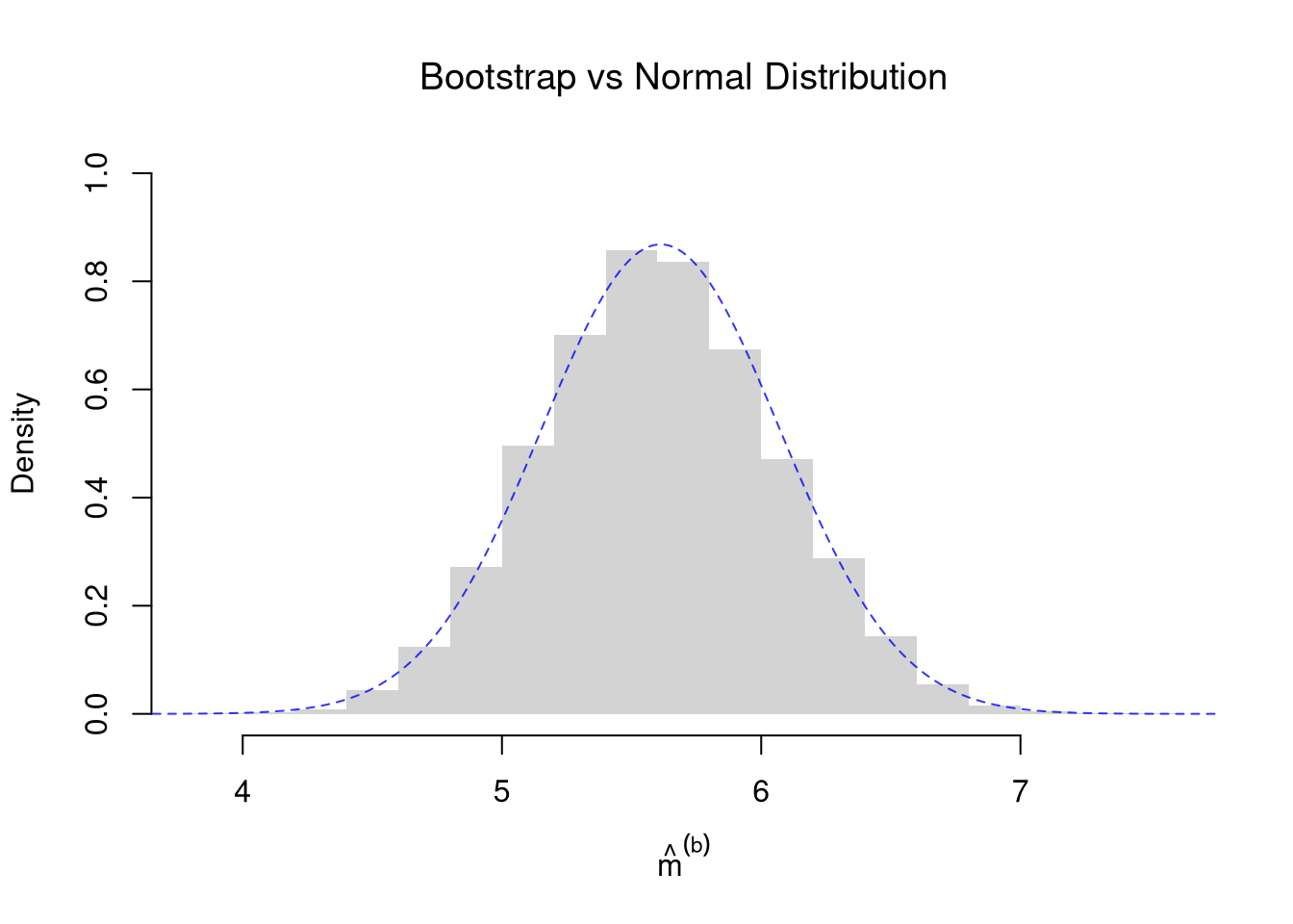
Another data-driven way is to create a bootstrap distribution for the sample mean and then compute the standard deviation of the bootstrap distribution \(\hat{\text{SE}}^{\text{boot}} \approx \text{SE}(M)\), as shown in Sampling & Resampling. The theory-driven estimate can differ from the bootstrap estimate in a finite sample, although both methods here assume i.i.d. observations. The standard error formula does not require normality. The theory-driven estimate does have some advantages too, but we do not go into that as we would need more advanced mathematics.
To compare the two, take another sample from the pretend population, as if it were all we observed.
Code
## MAIN EXAMPLE
# One sample of 50 workers, as if it were all we observed
x_sim <- sample(population_wages, 50, replace=FALSE)
n <- length(x_sim)
s_hat <- sqrt(mean((x_sim - mean(x_sim))^2)) # divides by n, unlike sd()
theory_se <- s_hat/sqrt(n)

# Bootstrap estimates
boot_means_wage <- rep(NA, 9999)
for(b in seq_along(boot_means_wage)){
    x_boot <- sample(x_sim, replace=TRUE) # c.f. jackknife
    m_b_hat <- mean(x_boot)
    boot_means_wage[b] <- m_b_hat
}
boot_se <- sd(boot_means_wage)

# Compare SE's
paste0('Bootstrap SE = ', round(boot_se, 3))
## [1] "Bootstrap SE = 0.458"
paste0('Class SE = ', round(theory_se, 3))
## [1] "Class SE = 0.459"
paste0('True SE = ', round(sqrt(population_wage_var/n), 3))
## [1] "True SE = 0.462"
Both estimates use only the one sample. We can compute the true standard error only because we pretend to know the population.
Shape
Sometimes, the sampling distribution is approximately normal due to the CLT. For a sufficiently large sample of i.i.d. observations with finite positive variance, \(M\) is approximately normal with mean \(\mathbb{E}[X_{i}]\) and standard deviation \(\text{SE}(M)=\sqrt{\mathbb{V}[X_{i}]/n}\). We estimate this standard error with \(\hat{s}/\sqrt{n}\).
Code
# Bootstrap Distribution
hist(boot_means_wage, breaks=25,
    main=NA, border=NA,
    freq=FALSE, ylim=c(0, 1),
    xlab=expression(hat(m)^group('(', b, ')')))
title('Bootstrap vs Normal Distribution', font.main=1)

# Theoretical Distribution: Normal Approximation with IID SEs
x <- seq(3, 9, by=0.01)
fx <- dnorm(x, mean(x_sim), theory_se)
lines(x, fx, col=rgb(0, 0, 1, .8), lty=2)
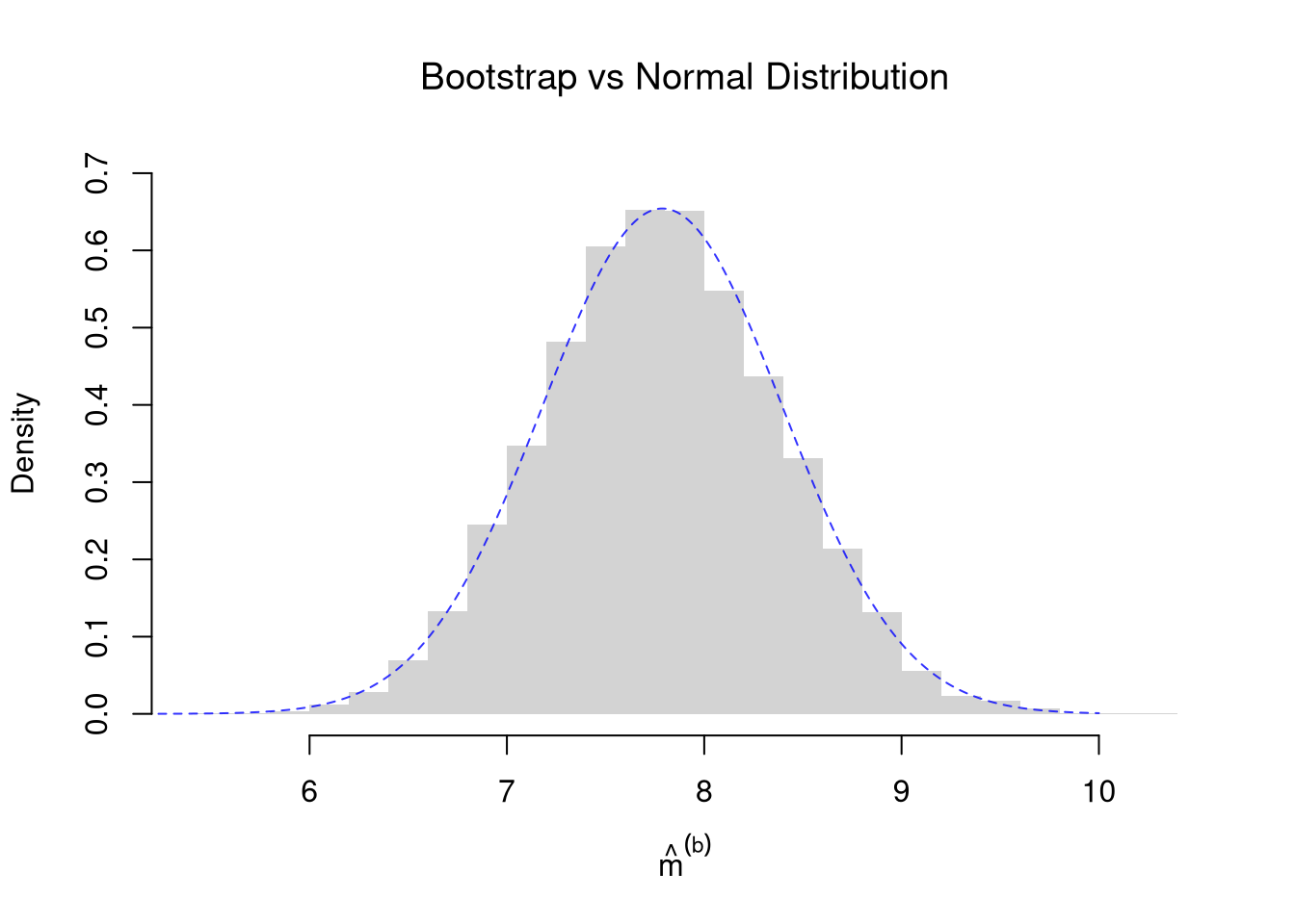
Repeat the comparison with murder arrests in USArrests. With no known population, there is no true standard error to compare with.
Code
# These 50 US states are one sample, with no known population.
x2_hat <- USArrests[, 'Murder'] # murder arrests per 100,000
n2 <- length(x2_hat)
s2_hat <- sqrt(mean((x2_hat - mean(x2_hat))^2)) # divides by n, unlike sd()
theory_se2 <- s2_hat/sqrt(n2)

# Bootstrap estimates
boot_means2 <- rep(NA, 9999)
for(b in seq_along(boot_means2)){
    x_boot <- sample(x2_hat, replace=TRUE)
    m_b_hat <- mean(x_boot)
    boot_means2[b] <- m_b_hat
}
boot_se2 <- sd(boot_means2)

# Compare SE's
paste0('Bootstrap SE = ', round(boot_se2, 3))
## [1] "Bootstrap SE = 0.603"
paste0('Class SE = ', round(theory_se2, 3))
## [1] "Class SE = 0.61"

# Bootstrap Distribution
hist(boot_means2, breaks=25,
    main=NA, border=NA,
    freq=FALSE, ylim=c(0, 0.7),
    xlab=expression(hat(m)^group('(', b, ')')))
title('Bootstrap vs Normal Distribution', font.main=1)

# Theoretical Distribution: Normal Approximation with IID SEs
x <- seq(5, 10, by=0.01)
fx <- dnorm(x, mean(x2_hat), theory_se2)
lines(x, fx, col=rgb(0, 0, 1, .8), lty=2)
Law of the Unconscious Statistician (LOTUS)
The variance estimator \(V=\sum_{i=1}^{n}(X_{i}-M)^2/n\) is nearly a sample mean of the squared deviations \(Y_{i}=(X_{i}-\mathbb{E}[X_{i}])^2\). So in large samples, the CLT says \(V\) is approximately normal, with a center and spread set by the mean and variance of \(Y_{i}\). We often care about a transformed quantity like \(Y_{i}\) or \(\log(X_{i})\), and would prefer not to derive its full distribution from scratch just to take its expectation. The Law of the Unconscious Statistician (LOTUS) gives the expected value of a function of a random variable without first deriving the distribution of that function. For discrete \(X_{i}\) and any function \(g\), \[\mathbb{E}[g(X_{i})] = \sum_{x} g(x) \text{Prob}(X_{i}=x).\] For continuous \(X_{i}\), replace the sum with an integral against \(f(x)\). LOTUS is useful as a shortcut: instead of deriving the distribution of \(g(X_{i})\) and then summing \(y \cdot \text{Prob}(g(X_{i}) = y)\), we sum \(g(x) \cdot \text{Prob}(X_{i}=x)\) directly using the original distribution of \(X_{i}\). You have already seen the special case \(g(X_{i})=\left(X_{i}-\mathbb{E}[X_{i}]\right)^2\), which is the population variance. The plug-in principle applies here too: putting \(\hat{p}(x)\) into LOTUS estimates \(\mathbb{E}[g(X_{i})]\) with \(\sum_{x} g(x)\hat{p}(x)\), which is the sample mean of the \(g(\hat{x}_{i})\). With \(g(x)=(x-\mathbb{E}[X_{i}])^2\), this is the average squared deviation from the population mean, and \(V\) differs from it only by using \(M\) in place of \(\mathbb{E}[X_{i}]\).
Let \(X_{i}\) take values \(\{1,2,3\}\) with \[
\text{Prob}(X_{i}=1)=0.2,\quad \text{Prob}(X_{i}=2)=0.5,\quad \text{Prob}(X_{i}=3)=0.3.
\] Let \(g(x)=x^2+1\). Then \(g(1)=1^2+1=2\), \(g(2)=2^2+1=5\), \(g(3)=3^2+1=10\).
Then, by LOTUS, \[\begin{aligned}
\mathbb E[g(X_{i})]=\sum_{x} g(x)\text{Prob}(X_{i}=x)
&= g(1)\cdot 0.2 + g(2)\cdot 0.5 + g(3)\cdot 0.3 \\
&= 2 \cdot 0.2 + 5 \cdot 0.5 + 10 \cdot 0.3 \\
&= 0.4 + 2.5 + 3 = 5.9.
\end{aligned}\]
Code
x  <- c(1, 2, 3)
x_probs <- c(0.2, 0.5, 0.3)
g  <- function(x) x^2 + 1
sum(g(x) * x_probs)
## [1] 5.9
For a fair four-sided die and \(g(x)=x^2+1\), LOTUS gives \(\mathbb{E}[g(X_{i})]\) exactly, and a simulation gives nearly the same number.
Code
g  <- function(x) x^2 + 1

# A theoretical example
x <- c(1, 2, 3, 4)
x_probs <- c(1/4, 1/4, 1/4, 1/4)
sum(g(x) * x_probs)
## [1] 8.5

# A simulation example
x_sim <- sample(x, prob=x_probs, size=1000, replace=TRUE)
mean(g(x_sim))
## [1] 8.348
Economists often work with logged data. LOTUS gives the population mean of the logged values directly from the original distribution, with \(g(x)=\log(x)\).
Code
## MAIN EXAMPLE
# E[log(X)] by LOTUS
sum(log(population_wages) * wage_probs)
## [1] 1.587268
# The population mean of log wages is 1.59.

# log(E[X]) is a different number
log(population_wage_mean)
## [1] 1.750518
# The log of the population mean wage is 1.75, so the two numbers differ.
In general, \(\mathbb{E}[g(X_{i})] \neq g(\mathbb{E}[X_{i}])\), so you cannot compute the expected value first and transform it afterwards.
If \(X_{i}\) is a continuous random variable (a random variable with a continuous sample space) and \(g\) is a function, then \(\mathbb E[g(X_{i})] = \int_{-\infty}^{\infty} g(x)f(x) dx\).
Code
x_sim <- rexp(5e5, rate = 1)           # X ~ Exp(1)
mean(sqrt(x_sim))                      # LOTUS Simulation
## [1] 0.8857528
sqrt(pi) / 2                       # Exact via LOTUS integral
## [1] 0.8862269
The variance estimator \(V=\sum_{i=1}^{n}(X_{i}-M)^2/n\) also has a sampling distribution. Write \(Y_{i}=g(X_{i})=(X_{i}-\mathbb{E}[X_{i}])^2\) for the squared deviation of each observation from the population mean. Expanding the square, and using \(\sum_{i=1}^{n}(X_{i}-\mathbb{E}[X_{i}])/n = M-\mathbb{E}[X_{i}]\), \[\begin{aligned}
V &= \frac{1}{n}\sum_{i=1}^{n} \left( [X_{i}-\mathbb{E}[X_{i}]] - [M-\mathbb{E}[X_{i}]] \right)^2 \\
&= \frac{1}{n}\sum_{i=1}^{n} Y_{i} - 2\left(M-\mathbb{E}[X_{i}]\right)^2 + \left(M-\mathbb{E}[X_{i}]\right)^2 \\
&= \frac{1}{n}\sum_{i=1}^{n} Y_{i} - \left(M-\mathbb{E}[X_{i}]\right)^2.
\end{aligned}\] So \(V\) is a sample mean of the \(Y_{i}\) minus a correction term. By LOTUS, each \(Y_{i}\) has mean \(\mathbb{E}[Y_{i}]=\mathbb{V}[X_{i}]\) and variance \(\mathbb{V}[Y_{i}]=\mathbb{E}[(X_{i}-\mathbb{E}[X_{i}])^4]-\mathbb{V}[X_{i}]^2\). The correction term has mean \(\mathbb{E}[(M-\mathbb{E}[X_{i}])^2]=\mathbb{V}[M]=\mathbb{V}[X_{i}]/n\), so \(\mathbb{E}[V]=\frac{n-1}{n}\mathbb{V}[X_{i}]\). The correction term shrinks like \(1/n\), faster than the \(1/\sqrt{n}\) standard error of the sample mean of the \(Y_{i}\). So the CLT applied to the \(Y_{i}\) says that, in large samples, \(V\) is approximately normal with mean \(\mathbb{V}[X_{i}]\) and standard error \(\text{SE}(V)=\sqrt{\mathbb{V}[Y_{i}]/n}\).
For the five-sided die, LOTUS gives \(\mathbb{V}[X_{i}]=2\) and \(\mathbb{E}[(X_{i}-3)^4]=(16+1+0+1+16)/5=34/5\), so \(\mathbb{V}[Y_{i}]=34/5-2^2=14/5\). With \(n=100\) rolls, \(\mathbb{E}[V]=\frac{99}{100} \times 2=\frac{99}{50}\) and \(\text{SE}(V)=\sqrt{\frac{14/5}{100}}=\sqrt{\frac{7}{250}}\approx 0.167\).
Code
# Five-sided die: population moments by LOTUS
x <- c(1, 2, 3, 4, 5)
x_probs <- rep(1/5, 5)
population_mean <- sum(x * x_probs)
population_var <- sum((x - population_mean)^2 * x_probs) # E[Y_i]
population_m4 <- sum((x - population_mean)^4 * x_probs) # E[(X_i - E[X_i])^4]
y_var <- population_m4 - population_var^2 # V[Y_i]

# Sampling distribution of V across many samples of n rolls
n <- 100
sample_vars <- rep(NA, 2000)
for(i in seq_along(sample_vars)){
    x_sim <- sample(x, prob=x_probs, size=n, replace=TRUE)
    v_hat <- mean((x_sim - mean(x_sim))^2) # divide-by-n variance
    sample_vars[i] <- v_hat
}
round(mean(sample_vars), 3) # near (n-1)/n * 2 = 1.98
## [1] 1.986
round(sd(sample_vars), 3) # near sqrt(2.8/n) = 0.167
## [1] 0.17

hist(sample_vars, breaks=25,
    border=NA, freq=FALSE, ylim=c(0, 2.6),
    xlab=expression(hat(v)),
    main=NA)
title('Sampling Distribution of the Variance', font.main=1)

# CLT approximation, with the SE from LOTUS
v <- seq(1, 3, by=0.01)
fv <- dnorm(v, population_var, sqrt(y_var/n))
lines(v, fv, col=rgb(0, 0, 1, .8), lty=2)
Try it yourself with \(n=10\) rolls. Is the normal approximation still good?
Bias and Consistency
Knowing an estimator’s sampling distribution lets us judge how good the estimator is.
Bias
A natural first question is whether an estimator is right on average. The bias of an estimator is its expected value minus the parameter it targets. For the sample mean, \(\text{Bias}(M) = \mathbb{E}[M] - \mathbb{E}[X_{i}]\). An estimator is unbiased if its bias is zero.
Bias is useful for separating two reasons an estimate can miss its target: bad luck in one sample, which averages out across samples, and a systematic error, which does not. From Means, \(\mathbb{E}[M]=\mathbb{E}[X_{i}]\), so the sample mean is unbiased.
The variance estimator \(V=\sum_{i=1}^{n}(X_{i}-M)^2/n\) is biased, because \(\mathbb{E}[V]=\frac{n-1}{n}\mathbb{V}[X_{i}]\). So we often use the adjusted sample standard deviation in theoretical calculations, \[
\hat{s}_{\text{adj}} = \sqrt{\frac{\sum_{i=1}^{n} (\hat{x}_{i} - \hat{m})^2}{n-1}},
\] which divides by \(n-1\) instead of \(n\). R’s sd() computes \(\hat{s}_{\text{adj}}\), and var() computes its square.
The variance estimator is \(V=\sum_{i=1}^{n}(X_{i}-M)^2/n\), which is biased; \(\text{Bias}(V) = \mathbb{E}[V] - \mathbb{V}[X_{i}]\). On average, it is too small by a factor of \(\frac{n-1}{n}\), \[\begin{aligned}
\mathbb{E}[V] &= \frac{n-1}{n}\mathbb{V}[X_{i}] \\
\text{Bias}(V) &= -\frac{\mathbb{V}[X_{i}]}{n}.
\end{aligned}\] The reason is that \(V\) measures deviations from the sample mean, which sits at the center of its own sample. In total, the observations are closer to it than to the population mean, so the squared deviations come out too small. This is why the adjusted version in Summary Statistics, which divides by \(n-1\), is called unbiased. The Test Yourself in LOTUS derives the formula. The bias shrinks as \(n\) grows.
The pretend population lets us check this with samples of \(n=10\) observations, where the bias is a tenth of the population variance.
Code
# Many samples of 10 workers
n <- 10
wage_vars <- rep(NA, 10000)
for(i in seq_along(wage_vars)){
    x_sim <- sample(population_wages, n, replace=FALSE)
    v_hat <- mean((x_sim - mean(x_sim))^2) # divide-by-n variance
    wage_vars[i] <- v_hat
}
round(mean(wage_vars), 2) # average estimate across samples
## [1] 9.6
round((n-1)/n*population_wage_var, 2) # E[V] from the formula
## [1] 9.62
round(population_wage_var, 2) # population variance
## [1] 10.68
# The average estimate, about 9.6, is close to E[V] from the formula, 9.62.
# It is not close to the population variance, 10.68.
Now return to the two fair coin flips in Statistical Theory, where \(\mathbb{V}[X_{i}]=\frac{1}{2} \times \frac{1}{2}=\frac{1}{4}\). In each of the four samples, compute \(V=[(X_{1}-M)^2+(X_{2}-M)^2]/2\): \[\begin{aligned}
\text{HH}: \quad V &= [(1-1)^2+(1-1)^2]/2 = 0 \\
\text{HT}: \quad V &= [(1-\frac{1}{2})^2+(0-\frac{1}{2})^2]/2 = 1/4 \\
\text{TH}: \quad V &= [(0-\frac{1}{2})^2+(1-\frac{1}{2})^2]/2 = 1/4 \\
\text{TT}: \quad V &= [(0-0)^2+(0-0)^2]/2 = 0.
\end{aligned}\] Each sample has probability \(1/4\), so \[\begin{aligned}
\mathbb{E}[V] &= 0 \times \frac{1}{4} + \frac{1}{4} \times \frac{1}{4} + \frac{1}{4} \times \frac{1}{4} + 0 \times \frac{1}{4} = \frac{1}{8} \\
\text{Bias}(V) &= \frac{1}{8} - \frac{1}{4} = -\frac{1}{8},
\end{aligned}\] which matches \(-\mathbb{V}[X_{i}]/n = -\frac{1}{4}/2 = -\frac{1}{8}\).
Code
# The four samples HH, HT, TH, TT, each with probability 1/4
x1 <- c(1, 1, 0, 0) # first flip
x2 <- c(1, 0, 1, 0) # second flip
x_probs <- c(1/4, 1/4, 1/4, 1/4)
m_samples <- (x1 + x2)/2
v_samples <- ((x1 - m_samples)^2 + (x2 - m_samples)^2)/2
v_samples
## [1] 0.00 0.25 0.25 0.00

sum(v_samples * x_probs) # E[V]
## [1] 0.125
sum(v_samples * x_probs) - 1/4 # Bias(V)
## [1] -0.125
Consistency
Bias describes an estimator at one sample size, so a natural next question is what happens as we collect more data. An estimator is consistent if its estimates get closer and closer to the parameter it targets as the sample grows. With enough data, nearly every sample gives an estimate close to the parameter.
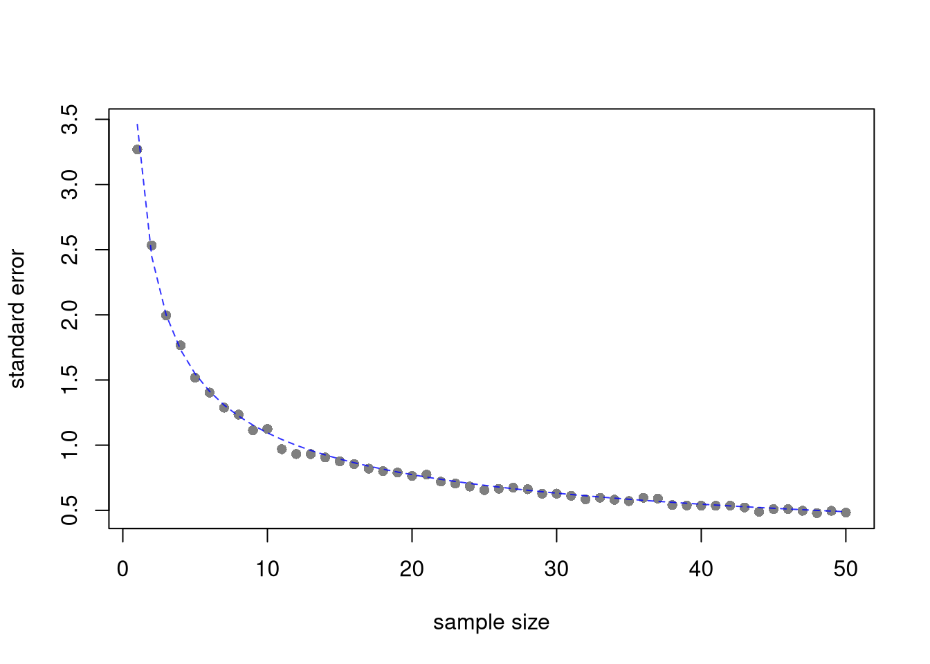
Consistency is useful as a minimum requirement: an estimator that is not consistent can stay wrong no matter how much data we collect. The Law of Large Numbers says that the sample mean is consistent. The reason is the shrinking standard error from Variances. As \(\text{SE}(M)=\sqrt{\mathbb{V}[X_{i}]/n}\) falls toward zero, the sampling distribution of \(M\) piles up around \(\mathbb{E}[X_{i}]\).
Note that each additional data point you have provides more information, which ultimately decreases the standard error of your estimates. This is why statisticians will often recommend that you get more data. However, the \(1/\sqrt{n}\) rate means each additional data point lowers the standard error by less than the one before. In economics, this is known as diminishing returns, and it is why economists may recommend you do not get more data.
Code
## MAIN EXAMPLE
# One sample of 50 workers, as if it were all we observed
x_sim <- sample(population_wages, 50, replace=FALSE)

n_boot <- 999 # number of bootstrap samples
sample_sizes <- seq(1, length(x_sim), by=1) # different resample sizes

## For each sample size, compute the bootstrap SE
se_by_n <- rep(NA, length(sample_sizes))
for(n in seq_along(sample_sizes)){
    boot_means_n <- rep(NA, n_boot)
    for(b in seq(1, n_boot)){
        x_boot <- sample(x_sim, size=n, replace=TRUE)
        m_b_hat <- mean(x_boot) # statistic of interest
        boot_means_n[b] <- m_b_hat
    }
    se_n <- sd(boot_means_n) # How much the statistic varies across samples
    se_by_n[n] <- se_n
}

# Theory-driven standard error at each sample size, with s_adj in place of the population SD
se_theory_n <- sd(x_sim)/sqrt(sample_sizes)

plot(sample_sizes, se_by_n, pch=16, col=grey(0, 0.5),
    ylim=range(c(se_by_n, se_theory_n)),
    ylab='standard error', xlab='sample size', main=NA)
lines(sample_sizes, se_theory_n, col=rgb(0, 0, 1, .8), lwd=1, lty=2)
With the pretend population, we can watch this happen. The chunk below records how often the sample mean misses the population mean by a fixed amount.
Code
# Share of 2000 samples whose mean misses by one dollar or more
n_values <- c(10, 50, 250)
miss_share <- rep(NA, length(n_values))
for(ni in seq_along(n_values)){
    wage_means_n <- rep(NA, 2000)
    for(i in seq_along(wage_means_n)){
        x_sim <- sample(population_wages, n_values[ni], replace=FALSE)
        wage_means_n[i] <- mean(x_sim)
    }
    miss_share[ni] <- mean(abs(wage_means_n - population_wage_mean) >= 1)
}
round(cbind(n=n_values, share=miss_share), 3)
##        n share
## [1,]  10 0.314
## [2,]  50 0.024
## [3,] 250 0.000
# The share of samples that miss falls toward zero as n grows.
# It is about 31% with n=10, about 2% with n=50, and about 0% with n=250.
Consistency does not require an unbiased estimator. The variance estimator \(V\) is biased, but both its bias and its spread shrink as \(n\) grows, so \(V\) is consistent too. The reverse also happens. The first observation \(X_{1}\) is an unbiased estimator of \(\mathbb{E}[X_{i}]\), but it is not consistent, because its distribution does not change as \(n\) grows.
Exercises
Comment the script you wrote for this chapter, then restart R and check that it runs from a clean session, then check the script with AI as explained in Working with AI. Write three sentences from memory on the main statistical idea of this chapter, and ask the assistant what is wrong, vague, or missing. Finish with your own questions about whatever you found hardest.
Explain in your own words the difference between an estimate \(\hat{m}\), an estimator \(M\), and a population parameter \(\mathbb{E}[X_{i}]\). Why is it important to distinguish between these three concepts?
Suppose \(X_{i}\) is a discrete random variable with outcomes \(\{1, 3, 5, 7\}\) and corresponding probabilities \(\{0.1, 0.2, 0.4, 0.3\}\). Compute the theoretical mean \(\mathbb{E}[X_{i}]\), variance \(\mathbb{V}[X_{i}]\), and standard deviation \(\sqrt{\mathbb{V}[X_{i}]}\) by hand. Verify your answers using R.
Using the USArrests dataset in R, compute the sample mean and the bootstrap standard error of the mean for the Assault variable. Then compute the theory-driven standard error \(\hat{s}/\sqrt{n}\) and compare the two estimates.
Using the Wages1 population, draw many samples of \(n=5\) workers and compute the bias of the variance estimator \(V\). Compare it with the formula \(-\mathbb{V}[X_{i}]/n\). Repeat with \(n=50\).
Recall
We defined population parameters, \(\mathbb{E}[X_{i}]\) and \(\mathbb{V}[X_{i}]\), and their estimators, \(M\) and \(V\). We also covered linearity of expectation and LOTUS. The standard error of the sample mean shrinks at the \(1/\sqrt{n}\) rate. The five-sided die computation made the parameters concrete: with outcomes \(\{1, 2, 3, 4, 5\}\) each having probability \(1/5\), the population mean is \(\mathbb{E}[X_{i}] = 15/5 = 3\) and the variance is \(\mathbb{V}[X_{i}] = (4+1+0+1+4)/5 = 2\). The \(1/\sqrt{n}\) rule then says that if a population has standard deviation \(10\), samples of size \(n=4\) have \(\text{SE}(M) = 5\) but quadrupling the sample size to \(n=16\) halves the standard error to \(2.5\). An estimator’s bias is its expected value minus its target. For two fair coin flips, the divide-by-\(n\) variance has \(\mathbb{E}[V]=1/8\) against a target of \(\mathbb{V}[X_{i}]=1/4\), so its bias is \(-1/8\). So we often use the adjusted sample standard deviation \(\hat{s}_{\text{adj}}\), which divides by \(n-1\). An estimator is consistent if its estimates get closer and closer to the parameter it targets as the sample grows. In the wage population, the share of samples whose mean missed by a dollar or more fell from about 31% with \(10\) workers to almost none with \(250\).