21  Multivariate Distributions


Most datasets record more than two variables for each observation. A worker has a wage, years of schooling, years of experience, and a sex.

This chapter asks three questions.

The recurring lesson is that a comparison between two variables can look different once a third variable is held fixed. The only prerequisites are the data frames, proportions, ECDFs, and boxplots from Data & Visualization, and the scatterplot from Bivariate Distributions.

21.1 Discrete Data

Three-Way Tables

Joint Distributions tabulated two discrete variables at once. With three, the table gains a third dimension.

ImportantKey Definition

The joint distribution of three discrete variables \(\hat{x}_{i}\), \(\hat{y}_{i}\), and \(\hat{z}_{i}\) is the share of observations with each combination of values: \[\hat{p}(x,y,z) = \sum_{i=1}^{n}\mathbf{1}\left( \hat{x}_{i}=x, \hat{y}_{i}=y, \hat{z}_{i}=z \right)/n.\] Summing over the values of one variable collapses the table to the two-way joint distribution of the other two, for example \(\hat{p}(x,y) = \sum_{z} \hat{p}(x,y,z)\).

A three-way table is useful whenever a two-way comparison might depend on a third factor. It keeps every combination visible. Collapsing it recovers the two-way table you would have made had you ignored the third variable. R can store counts directly as a three-way table, such as the built-in UCBAdmissions.

Code
## MAIN EXAMPLE
# UCBAdmissions counts graduate applications to six Berkeley departments in 1973.
# Three factors: Admit (2 levels), Gender (2 levels), Dept (6 levels)
dim(UCBAdmissions)
## [1] 2 2 6
dimnames(UCBAdmissions)
## $Admit
## [1] "Admitted" "Rejected"
## 
## $Gender
## [1] "Male"   "Female"
## 
## $Dept
## [1] "A" "B" "C" "D" "E" "F"

# ftable() flattens the table so it prints on one page
ftable(UCBAdmissions, row.vars=c('Dept', 'Gender'), col.vars='Admit')
##             Admit Admitted Rejected
## Dept Gender                        
## A    Male              512      313
##      Female             89       19
## B    Male              353      207
##      Female             17        8
## C    Male              120      205
##      Female            202      391
## D    Male              138      279
##      Female            131      244
## E    Male               53      138
##      Female             94      299
## F    Male               22      351
##      Female             24      317

Dividing by the total number of applicants gives the joint distribution, and margin.table() collapses it.

Code
# Joint distribution over all 24 cells
n <- sum(UCBAdmissions)
p_xyz <- UCBAdmissions / n

# Collapse over Dept to get the two-way distribution of Admit and Gender
p_xy <- margin.table(p_xyz, c(1, 2))
round(p_xy, 3)
##           Gender
## Admit       Male Female
##   Admitted 0.265  0.123
##   Rejected 0.330  0.282

# Collapse further to the marginal distribution of Gender
round(margin.table(p_xyz, 2), 3)
## Gender
##   Male Female 
##  0.595  0.405

Suppose \(n=20\) workers are recorded by sex (\(x\)), whether they were promoted (\(y\)), and whether they hold a degree (\(z\)).

Workers by Sex, Promotion, and Degree
No degree Degree
Men, promoted 2 4
Men, not promoted 6 2
Women, promoted 1 3
Women, not promoted 1 1

The joint proportion of promoted men without a degree is \(\hat{p}(\text{man}, \text{promoted}, \text{no degree}) = 2/20 = 0.10\). Collapsing over degree, the share of promoted men is \(\hat{p}(\text{man}, \text{promoted}) = (2+4)/20 = 0.30\). Collapsing again, the marginal share of men is \((2+6+4+2)/20 = 0.70\).

Code
# Build the same table from a small data frame, one row per worker
xy0_hat <- data.frame(
    sex=rep(c('man', 'woman'), c(14, 6)),
    degree=c(rep(c('no', 'yes'), c(8, 6)), rep(c('no', 'yes'), c(2, 4))),
    promoted=c(rep(c(1, 0), c(2, 6)), rep(c(1, 0), c(4, 2)),
        rep(c(1, 0), c(1, 1)), rep(c(1, 0), c(3, 1))))
tab <- table(xy0_hat)
ftable(tab, row.vars=c('sex', 'promoted'), col.vars='degree')
##                degree no yes
## sex   promoted              
## man   0                6   2
##       1                2   4
## woman 0                1   1
##       1                1   3

# Collapse over degree
round(margin.table(tab / sum(tab), c(1, 3)), 2)
##        promoted
## sex       0   1
##   man   0.4 0.3
##   woman 0.1 0.2

Conditional Proportions

Collapsing hides the third variable. Conditioning does the opposite: it fixes the third variable at one value and compares within that slice.

ImportantKey Definition

The conditional distribution of \(\hat{y}_{i}\) given \(\hat{x}_{i}=x\) and \(\hat{z}_{i}=z\) is the share of observations with \(\hat{y}_{i}=y\) inside the subgroup where both conditioning variables take the stated values: \[\hat{p}(y \mid x, z) = \frac{\hat{p}(x,y,z)}{\hat{p}(x,z)}.\]

Conditional proportions are useful for comparing groups on equal footing. For example, the admission rate for women in department A is compared with the rate for men in department A. So differences in which departments people apply to cannot drive the comparison. In R, prop.table() with a margin= argument divides each cell by the total of its slice.

Code
## MAIN EXAMPLE
# Admission rate by Gender, pooling all departments
p_pooled <- prop.table(margin.table(UCBAdmissions, c(1, 2)), margin=2)
round(p_pooled['Admitted', ], 2)
##   Male Female 
##   0.45   0.30
# Pooled over departments, men were admitted at a higher rate than women.

# Admission rate by Gender within each Dept
p_within <- prop.table(UCBAdmissions, margin=c(2, 3))
round(p_within['Admitted', , ], 2)
##         Dept
## Gender      A    B    C    D    E    F
##   Male   0.62 0.63 0.37 0.33 0.28 0.06
##   Female 0.82 0.68 0.34 0.35 0.24 0.07
# Women had higher rates than men in four of the six: A, B, D, and F.
# The gaps in D and F are small.
# Men had higher rates in C and E, so the reversal holds in most departments, not all.

The pooled and within-group tables are both correct summaries of the same data. They can differ when the slices differ in their rates and in their composition, which the pooled table mixes together. The code below computes both.

Code
# Where did each gender apply? Share of each gender's applications going to each Dept
p_apply <- prop.table(margin.table(UCBAdmissions, c(2, 3)), margin=1)
round(p_apply, 2)
##         Dept
## Gender      A    B    C    D    E    F
##   Male   0.31 0.21 0.12 0.15 0.07 0.14
##   Female 0.06 0.01 0.32 0.20 0.21 0.19
# Just over half of the men applied to departments A and B.
# Over 90% of the women applied to departments C to F.

# How selective is each Dept? Admission rate by Dept, pooling genders
p_dept <- prop.table(margin.table(UCBAdmissions, c(1, 3)), margin=2)
round(p_dept['Admitted', ], 2)
##    A    B    C    D    E    F 
## 0.64 0.63 0.35 0.34 0.25 0.06
# Departments A and B admitted over 60% of their applicants.
# Departments C to F admitted about 35% of their applicants or fewer.
# The pooled gap mostly reflects where people applied, not how they were treated.

The descriptive lesson is to report the within-group comparison alongside the pooled one, and say how the groups differ in composition.

Compute the number of applicants in each cell of the Gender by Dept table with margin.table(UCBAdmissions, c(2, 3)). Which two departments account for most of the male applicants, and what were their admission rates? Then verify that p_within can be rebuilt from the joint distribution as \(\hat{p}(x,y,z) / \hat{p}(x,z)\), using p_xyz and margin.table(p_xyz, c(2, 3)).

21.2 Continuous Data

Scatterplot Matrices

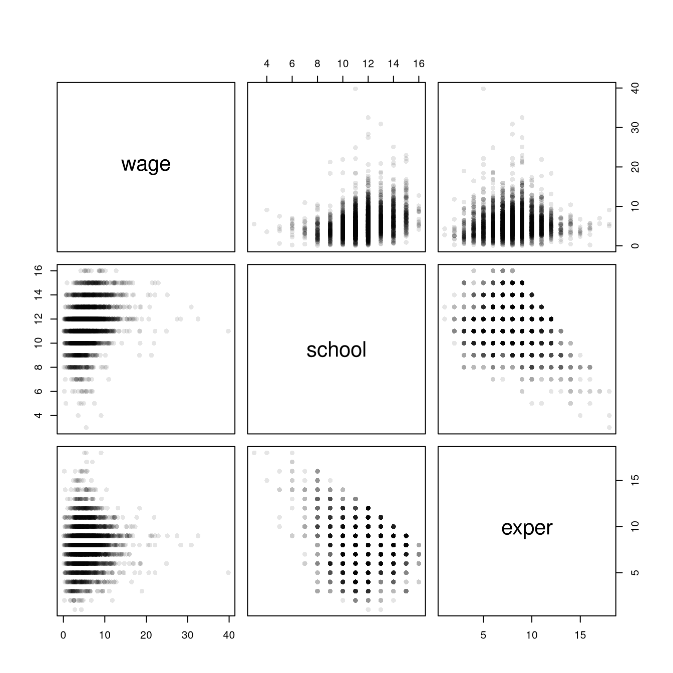
For two cardinal variables, the basic figure is the scatterplot: one point per observation, with \(\hat{x}_{i}\) on the horizontal axis and \(\hat{y}_{i}\) on the vertical axis. With several cardinal variables, there is one scatterplot for each pair. A scatterplot matrix draws all of them in one grid, so you can scan every pairwise relationship at once.

Code
## MAIN EXAMPLE
# Store the observed data, one row per worker
# The data cover 3294 US workers.
# wage is the hourly wage in 1980 dollars, and school and exper are in years.
data(Wages1, package='Ecdat')
xy_hat <- Wages1

# Every pair of the three cardinal variables, one panel each
pairs(xy_hat[, c('wage', 'school', 'exper')], pch=16, col=grey(0, .1), main=NA)

Code
# Row wage, column school plots wage (vertical) against schooling (horizontal).
# Schooling and experience are whole numbers, so their panels form stripes.
# More schooling goes with higher wages and with less experience.

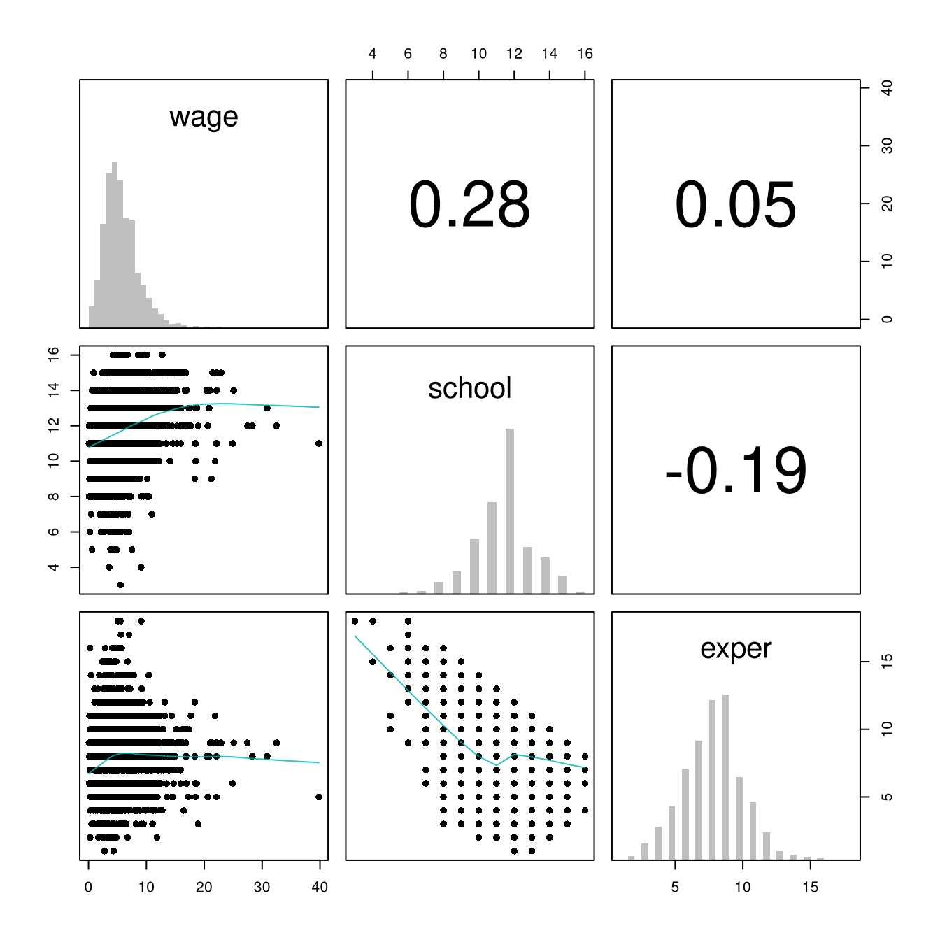
Each panel plots the variable named in its row on the vertical axis against the variable named in its column on the horizontal axis. The panel below the diagonal repeats the panel above it with the axes swapped, so you only need to read one triangle. The psych package adds histograms on the diagonal and a summary of each pairwise relationship in the upper triangle.

Code
# pairs.panels lays out univariate histograms on the diagonal,
# scatterplots in the lower triangle, and correlations in the upper triangle.
# With this many workers, smoother=TRUE shades each scatterplot by point density.
psych::pairs.panels(xy_hat[, c('wage', 'school', 'exper')],
    hist.col=grey(0, .25), breaks=30, density=FALSE, hist.border=NA, # Diagonal
    ellipses=FALSE, rug=FALSE, smoother=FALSE, pch=16, col=rgb(0, .7, .7, .8) # Lower Triangle
    )

Code
# Wages have a long right tail, and schooling piles up at 12 years.

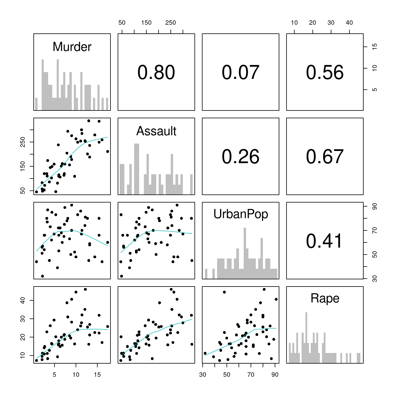
The diagonal shows univariate histograms. The lower triangle shows scatterplots between each pair of variables, shaded darker where observations pile up. The upper triangle shows correlation coefficients, a summary of linear association between \(-1\) and \(1\) that Associations defines. Scan the matrix for pairs where the cloud bends rather than running straight, and for points far from the rest of the cloud. Also look for pairs so tightly related that they carry almost the same information. Which pair of variables in Wages1 is most tightly related, and which pair is nearly unrelated?

Repeat the matrix with the USArrests data on US states. Which pair of variables is most tightly related, and which variable is nearly unrelated to the others?

Code
# 50 US states in 1973, with four cardinal variables, so there are six pairs.
# Murder, Assault, and Rape are arrests per 100,000 residents.
# UrbanPop is the percent of the population in urban areas.
xy2_hat <- USArrests

psych::pairs.panels(xy2_hat,
    hist.col=grey(0, .25), breaks=30, density=FALSE, hist.border=NA, # Diagonal
    ellipses=FALSE, rug=FALSE, smoother=FALSE, pch=16, col=rgb(0, .7, .7, .8) # Lower Triangle
    )

Code
# Row Murder, column Assault plots murder (vertical) against assault (horizontal).

Encoding More Variables

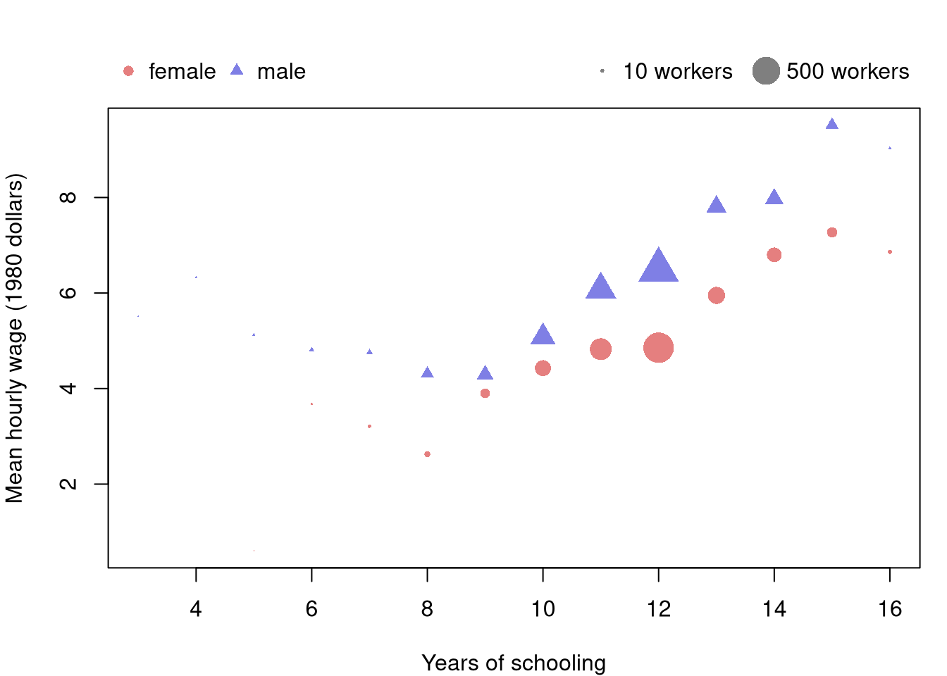
A scatterplot has two axes, but a point has more attributes than position: color, shape, and size can each carry another variable. With many observations the points overlap, so differences in size are hard to see. The figure below therefore draws one point for each combination of the horizontal variable and a factor, placed at the mean of the vertical variable. Color and shape mark the factor, and size marks how many observations the point summarizes.

Code
# One row per combination of schooling and sex: mean wage and number of workers
xy_cell_hat <- aggregate(wage ~ school + sex, data=xy_hat, FUN=mean)
xy_cell_hat$n_cell <- aggregate(wage ~ school + sex, data=xy_hat, FUN=length)$wage

# Color and shape mark sex
cols <- c(rgb(.8, 0, 0, .5), rgb(0, 0, .8, .5))
pchs <- c(16, 17)

# Point area scales with the number of workers
sizes <- sqrt(xy_cell_hat$n_cell / max(xy_cell_hat$n_cell)) * 3

# Legends go in the margin above the plot so they cover no points
par(mar=c(4, 4, 4, 1))
plot(wage ~ school, data=xy_cell_hat,
    pch=pchs[xy_cell_hat$sex], col=cols[xy_cell_hat$sex], cex=sizes,
    xlab='Years of schooling',
    ylab='Mean hourly wage (1980 dollars)', main=NA)
legend('topleft', inset=c(0, -.14), xpd=TRUE, horiz=TRUE, bty='n',
    legend=levels(xy_cell_hat$sex),
    pch=pchs, col=cols)
legend('topright', inset=c(0, -.14), xpd=TRUE, horiz=TRUE, bty='n',
    legend=c('10 workers', '500 workers'),
    pch=16, col=grey(0, .5), pt.cex=sqrt(c(10, 500) / max(xy_cell_hat$n_cell)) * 3)

Code
# Men's mean wage is above women's at all 12 schooling levels where both appear.
# Both means rise with schooling from 9 to 15 years.
# The largest points are at 12 years, with 594 workers of each sex.
# The smallest points hold only a few workers, so their means jump around.

Extra channels can show patterns that the plain panel of the matrix hid. Each added channel makes the figure harder to read, so two extra variables is a practical limit. Interactive versions, where hovering over a point reveals every variable at once, are covered in Communicating Results.

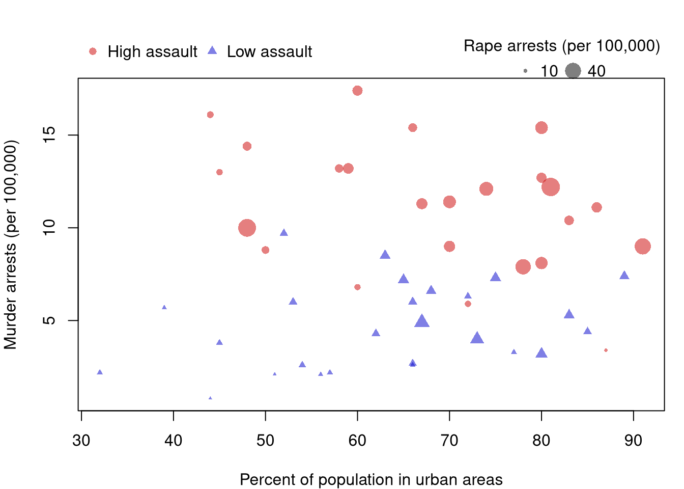
With few observations, each point can stand for one observation. Repeat the figure with USArrests, coloring and shaping each state by whether its assault rate is above the median, and sizing each point by its rape arrest rate.

Code
# 50 US states, so points overlap little and size can carry a fourth variable.
xy2_hat <- USArrests

# Split states at the median assault rate
assault2_high <- xy2_hat$Assault > median(xy2_hat$Assault)
col2_high <- rgb(.8, 0, 0, .5)
col2_low <- rgb(0, 0, .8, .5)
cols2 <- ifelse(assault2_high, col2_high, col2_low)
pchs2 <- ifelse(assault2_high, 16, 17)

# Scale point size by a fourth variable
sizes2 <- xy2_hat$Rape / max(xy2_hat$Rape) * 2.5

# Legends go in the margin above the plot so they cover no points
par(mar=c(4, 4, 4, 1))
plot(Murder ~ UrbanPop, data=xy2_hat, pch=pchs2, col=cols2, cex=sizes2,
    xlab='Percent of population in urban areas',
    ylab='Murder arrests (per 100,000)', main=NA)
legend('topleft', inset=c(0, -.14), xpd=TRUE, horiz=TRUE, bty='n',
    legend=c('High assault', 'Low assault'),
    pch=c(16, 17), col=c(col2_high, col2_low))
legend('topright', inset=c(0, -.14), xpd=TRUE, horiz=TRUE, bty='n',
    title='Rape arrests (per 100,000)', legend=c('10', '40'),
    pch=16, col=grey(0, .5), pt.cex=c(10, 40) / max(xy2_hat$Rape) * 2.5)

Code
# High-assault states sit toward the top at every level of urbanization.
# So the murder rate tracks the assault rate rather than the urban share.
# Larger points also cluster toward the top.
# So states with many murder arrests tend to have many rape arrests too.

21.3 Mixed Data

Conditioning Plots

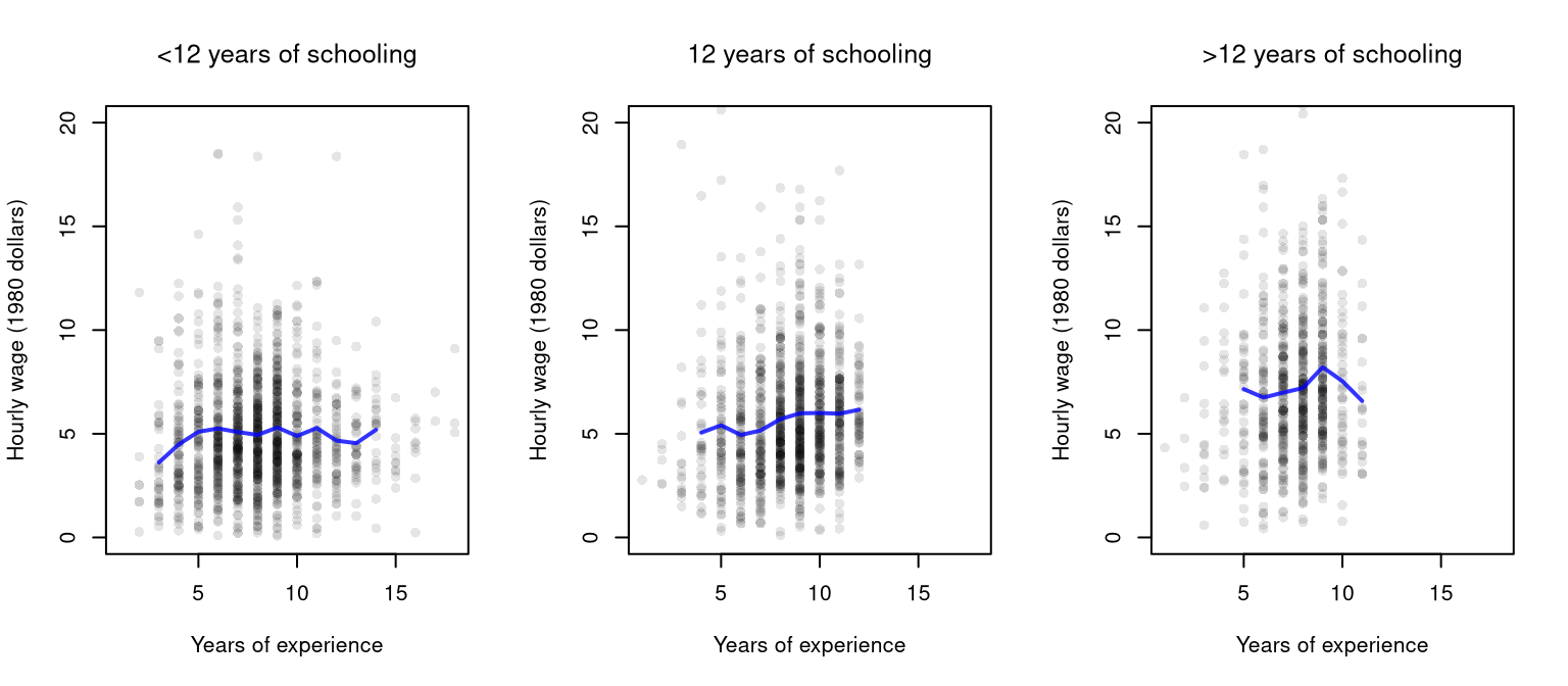
A scatterplot can also be split by a factor: draw it separately for each group. A conditioning plot holds the factor fixed within each panel, so any pattern that appears is a within-group pattern. Comparing Multiple Groups summarizes one factor at a time with boxplots and ECDFs; here we go straight to conditioning, and then combine two factors at once below.

Code
## MAIN EXAMPLE
# Three-level schooling factor, as in Comparing Multiple Groups
xy_hat$school_g <- cut(xy_hat$school, breaks=c(0, 11, 12, 16), labels=c('<12', '12', '>12'))

The line in each panel joins the group’s mean outcome across values of the horizontal variable, so the eye can follow the center of the cloud.

Code
## MAIN EXAMPLE
# One scatterplot per schooling group, on common axes to compare the panels
# Experience is on the horizontal axis, since the groups already use schooling.
# The wage axis ends just above 20 dollars, leaving out the 16 highest wages.
par(mfrow=c(1, 3))
for (g in levels(xy_hat$school_g)) {
    xy_g_hat <- xy_hat[xy_hat$school_g == g, ]
    plot(wage ~ exper, data=xy_g_hat, pch=16, col=grey(0, .1),
        xlim=range(xy_hat$exper), ylim=c(0, 20),
        xlab='Years of experience', ylab='Hourly wage (1980 dollars)', main=NA)
    title(paste0(g, ' years of schooling'), font.main=1)
    # Mean wage at each experience value held by 20 or more workers
    m_g_hat <- aggregate(wage ~ exper, data=xy_g_hat, FUN=mean)
    n_g <- table(xy_g_hat$exper)
    lines(wage ~ exper, data=m_g_hat[n_g >= 20, ], col=rgb(0, 0, 1, .8), lwd=2)
}

Code
# Pooled, wage and experience are nearly unrelated (correlation 0.05).
# Under 12 years: the mean wage stays near 5 dollars after 5 years of experience.
# Exactly 12 years: the mean wage rises from about 5 to about 6 dollars.
# Over 12 years: the mean wage is the highest at every experience value drawn.
# Its line also rises up to 9 years, then falls where few workers remain.

A pooled figure can hide within-group patterns like these when the groups differ in their averages.

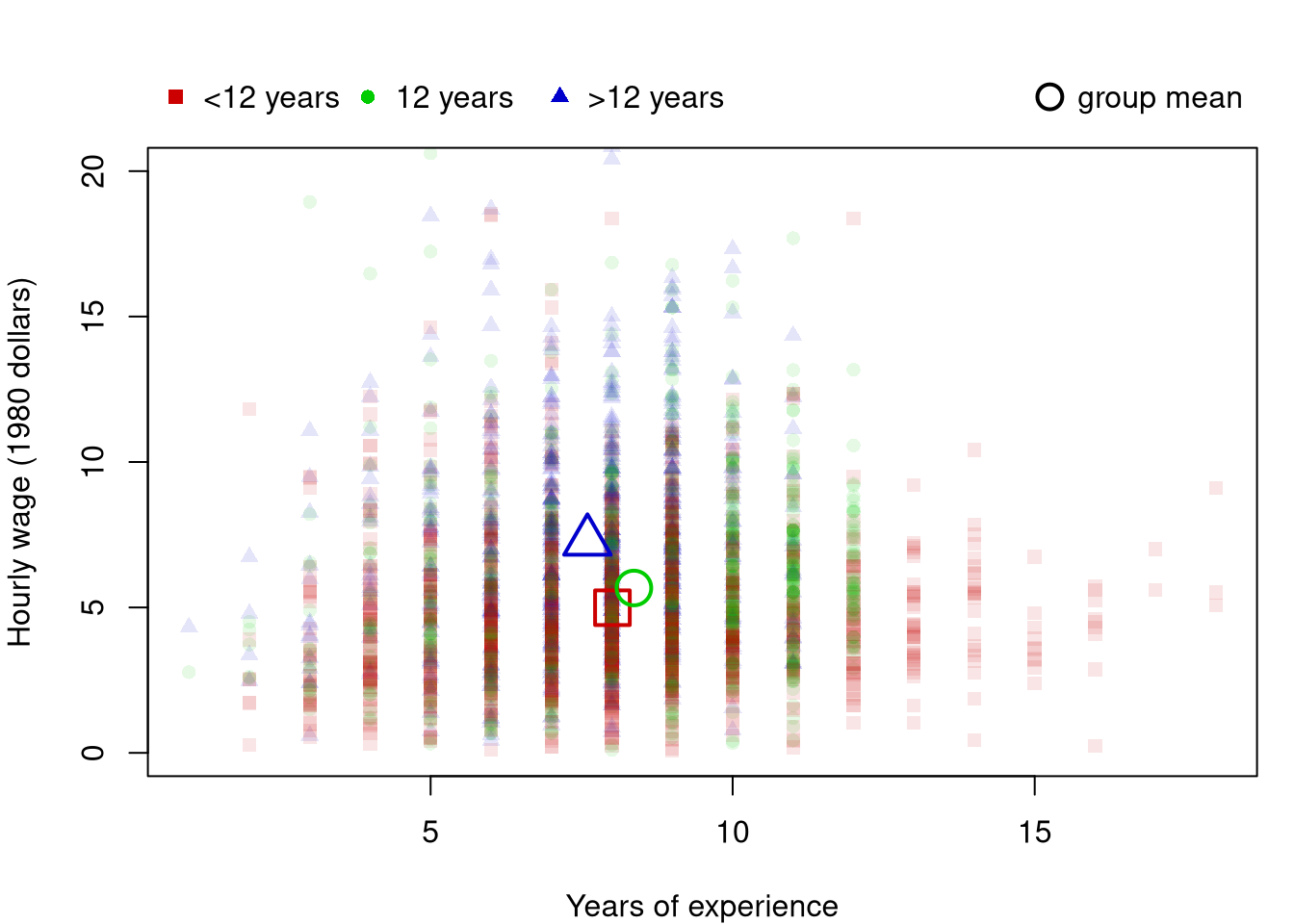
The pooled and within-group views can be placed on one figure. We mark each group with its own symbol and add each group’s center as a large hollow symbol. The hollow marker does not cover the observations beneath it.

Code
## MAIN EXAMPLE
# Small filled points: workers, by schooling; large hollow points: group means
# The wage axis ends just above 20 dollars, leaving out the 16 highest wages.
g_hues <- c(rgb(.8, 0, 0), rgb(0, .8, 0), rgb(0, 0, .8))
g_cols <- adjustcolor(g_hues, alpha.f=.1)
g_pch <- c(15, 16, 17)
g_pch_hollow <- c(0, 1, 2)
par(mar=c(4, 4, 4, 1))
plot(wage ~ exper, data=xy_hat, pch=g_pch[xy_hat$school_g], col=g_cols[xy_hat$school_g],
    ylim=c(0, 20),
    xlab='Years of experience', ylab='Hourly wage (1980 dollars)', main=NA)
means <- aggregate(cbind(exper, wage) ~ school_g, data=xy_hat, FUN=mean)
points(means$exper, means$wage, pch=g_pch_hollow, col=g_hues, cex=2.5, lwd=2)

# Legends in the margin above the plot
legend('topleft', inset=c(0, -.14), xpd=TRUE, horiz=TRUE, bty='n',
    legend=paste0(levels(xy_hat$school_g), ' years'), pch=g_pch, col=g_hues)
legend('topright', inset=c(0, -.14), xpd=TRUE, bty='n',
    legend='group mean', pch=1, col='black', pt.cex=1.8, pt.lwd=2)

Code
# The most-schooled group has the highest mean wage and the least experience.
# So the pooled cloud looks flatter than the panels with 12 or more years.
# Every worker with over 12 years of experience has under 12 years of schooling.

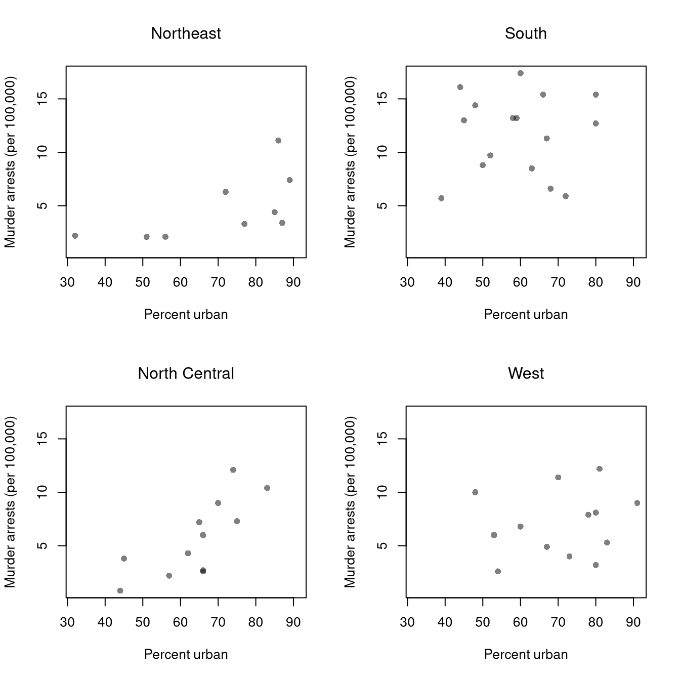
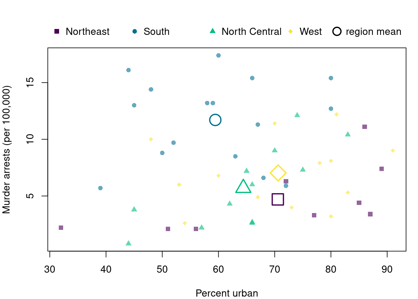
Repeat the conditioning plot and the overlay with USArrests, using one panel per census region.

Code
# 50 US states, with the four-level region factor attached
xy2_hat <- USArrests
xy2_hat$Region <- state.region

# One scatterplot per region, on common axes so the panels are comparable
par(mfrow=c(2, 2))
for (r in levels(xy2_hat$Region)) {
    xy2_r_hat <- xy2_hat[xy2_hat$Region == r, ]
    plot(Murder ~ UrbanPop, data=xy2_r_hat, pch=16, col=grey(0, .5),
        xlim=range(xy2_hat$UrbanPop), ylim=range(xy2_hat$Murder),
        xlab='Percent urban', ylab='Murder arrests (per 100,000)', main=NA)
    title(r, font.main=1)
}

Code
# Pooled over regions, murder rates are nearly unrelated to urbanization.
# In the Northeast and North Central, more urban states have higher murder rates.
# In the South and West there is little pattern.
# But the South sits high at every level of urbanization.
# The pooled figure hides the first two patterns.
# That is because the regions differ so much in their average murder rate.
Code
# Small filled points: states, by region; large hollow points: region means
region2_cols <- hcl.colors(4, alpha=.6)
region2_pch <- c(15, 16, 17, 18)
region2_pch_hollow <- c(0, 1, 2, 5)
par(mar=c(4, 4, 4, 1))
plot(Murder ~ UrbanPop, data=xy2_hat, pch=region2_pch[xy2_hat$Region], col=region2_cols[xy2_hat$Region],
    xlab='Percent urban', ylab='Murder arrests (per 100,000)', main=NA)
means2 <- aggregate(cbind(UrbanPop, Murder) ~ Region, data=xy2_hat, FUN=mean)
points(means2$UrbanPop, means2$Murder, pch=region2_pch_hollow, col=hcl.colors(4), cex=2.5, lwd=2)

# Legends in the margin above the plot
legend('topleft', inset=c(0, -.14), xpd=TRUE, horiz=TRUE, bty='n',
    legend=levels(xy2_hat$Region), pch=region2_pch, col=hcl.colors(4))
legend('topright', inset=c(0, -.14), xpd=TRUE, bty='n',
    legend='region mean', pch=1, col='black', pt.cex=1.8, pt.lwd=2)

Conditional means can reverse when pooled, for the same compositional reason as conditional proportions. Suppose \(40\) men and \(40\) women work at a firm, split by whether they hold a degree, with the mean hourly wage in each cell shown below.

Mean Hourly Wage by Sex and Degree
Men Women
No degree \(n=10\), mean \(10\) \(n=30\), mean \(11\)
Degree \(n=30\), mean \(20\) \(n=10\), mean \(21\)

Within each degree group, women earn \(1\) more per hour. Pooled, men earn \((10 \cdot 10 + 30 \cdot 20)/40 = 17.5\) and women earn \((30 \cdot 11 + 10 \cdot 21)/40 = 13.5\), so women earn \(4\) less. The pooled mean is a weighted average of the within-group means, \(\hat{m}_{Y}(x) = \sum_{z} \hat{m}_{Y}(x, z)\, \hat{p}(z \mid x)\). The weights differ by sex, since three quarters of the women and only one quarter of the men are in the no-degree group.

Code
# Rebuild the pooled means from the cell means and cell sizes
m_men_hat <- (10 * 10 + 30 * 20) / (10 + 30)
m_women_hat <- (30 * 11 + 10 * 21) / (30 + 10)
c(men=m_men_hat, women=m_women_hat)
##   men women 
##  17.5  13.5

Using xy_hat, draw a conditioning plot of wage against exper with one panel per sex. Use col=grey(0, .1), as in the panels above. Then compute the mean wage by sex, pooled and within each value of school, with aggregate(wage ~ sex + school, data=xy_hat, FUN=mean). Does the pooled gap match the within-schooling gaps?

Two Factors at Once

A group summary is not limited to one factor. Crossing two factors gives one group for each combination of levels, each smaller than the groups of either factor alone but still worth comparing.

Code
# Schooling group (3 levels) crossed with sex (2 levels) gives six groups
table(xy_hat$school_g, xy_hat$sex)
##      
##       female male
##   <12    567  786
##   12     594  594
##   >12    408  345
# Even the smallest group holds 345 workers.

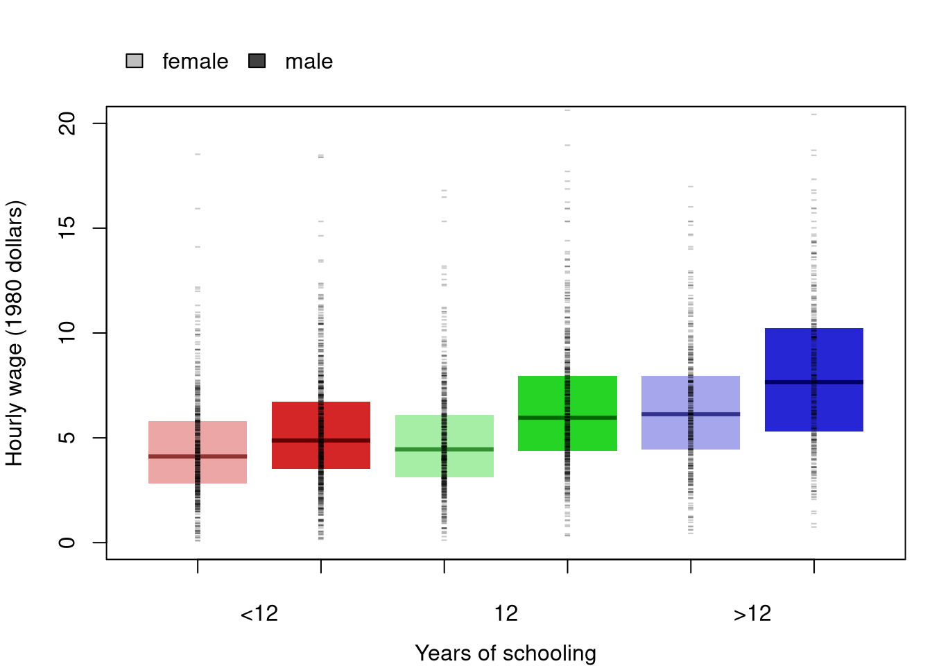
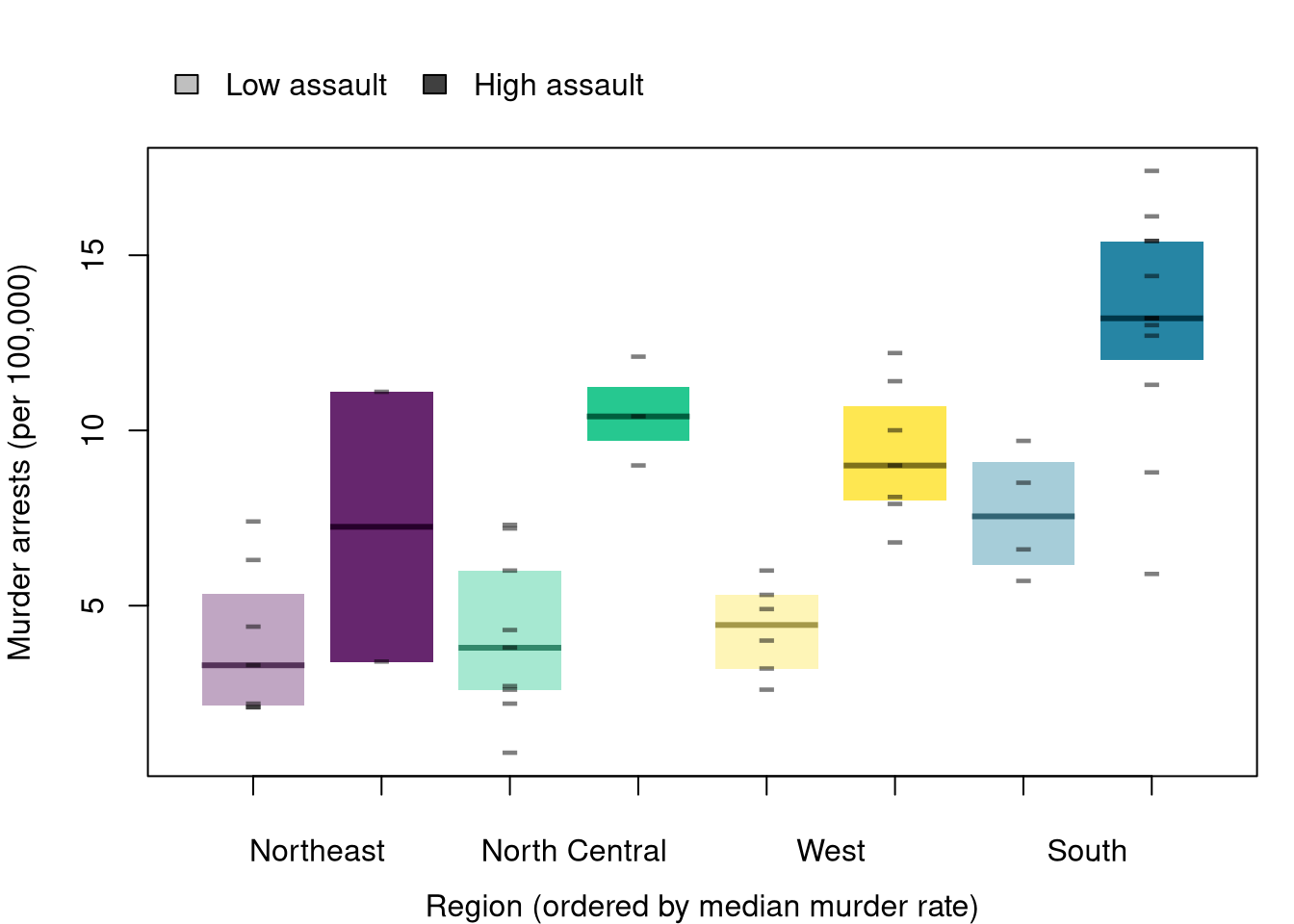
A grouped boxplot places the boxes for one factor side by side within each level of the other, so a within-group comparison and a between-group comparison are both visible at once. Color keeps the group hues used in Conditioning Plots above, and a lighter or darker shade of each hue marks the second factor, so hue and shade carry two different variables.

Code
## MAIN EXAMPLE
# Hue stays fixed to each schooling group; shade (light/dark) marks sex.
# Groups keep their own order, which also runs from low to high median wage.
col_f_shade <- adjustcolor(g_hues, alpha.f=.35)
col_m_shade <- adjustcolor(g_hues, alpha.f=.85)
box_cols <- as.vector(rbind(col_f_shade, col_m_shade))
med_cols <- adjustcolor(box_cols, alpha.f=2, red.f=.5, green.f=.5, blue.f=.5) # darker shades, for the medians

# The wage axis ends just above 20 dollars, leaving out the 16 highest wages.
par(mar=c(4, 4, 4, 1))
boxplot(wage ~ sex + school_g, data=xy_hat,
    col=box_cols, border=NA, medcol=med_cols, xaxt='n', ylim=c(0, 20),
    whisklty=0, staplelty=0, outline=FALSE,
    xlab='Years of schooling', ylab='Hourly wage (1980 dollars)', main=NA)
# Raw Observations, in place of whiskers and outliers
stripchart(wage ~ sex + school_g, data=xy_hat,
    pch='-', col=grey(0, .2), cex=1,
    vert=TRUE, add=TRUE)
axis(1, at=seq(1.5, by=2, length.out=3), labels=levels(xy_hat$school_g), tick=FALSE, line=0.5)
axis(1, at=seq_len(6), labels=FALSE)
legend('topleft', inset=c(0, -.16), xpd=TRUE, horiz=TRUE, bty='n',
    legend=levels(xy_hat$sex), fill=c(grey(.75), grey(.25)))

Code
# In every schooling group the median wage for men is above the median for women.

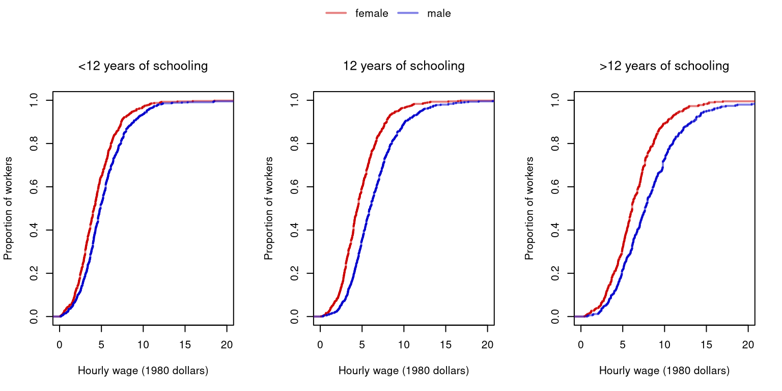
The same comparison as an ECDF, one panel per group, shows each full distribution as one curve rather than a box and dashes, with a single legend shared across all the panels.

Code
# One panel per schooling group; within each panel, one ECDF for each sex
# The wage axis ends just above 20 dollars, leaving out the 16 highest wages.
cols <- c(rgb(.8, 0, 0, .5), rgb(0, 0, .8, .5))
par(mfrow=c(1, 3), oma=c(0, 0, 3, 0))
for (g in levels(xy_hat$school_g)) {
    xy_g_hat <- xy_hat[xy_hat$school_g == g, ]
    plot(NULL, xlim=c(0, 20), ylim=c(0, 1),
        xlab='Hourly wage (1980 dollars)', ylab='Proportion of workers', main=NA)
    F_f_hat <- ecdf(xy_g_hat$wage[xy_g_hat$sex == 'female'])
    F_m_hat <- ecdf(xy_g_hat$wage[xy_g_hat$sex == 'male'])
    plot(F_f_hat, add=TRUE, col=cols[1], lwd=2, verticals=TRUE, do.points=FALSE, col.01line=NA)
    plot(F_m_hat, add=TRUE, col=cols[2], lwd=2, verticals=TRUE, do.points=FALSE, col.01line=NA)
    title(paste0(g, ' years of schooling'), font.main=1)
}

# One legend for all three panels, drawn on an invisible full-figure overlay
par(fig=c(0, 1, 0, 1), oma=c(0, 0, 0, 0), mar=c(0, 0, 0, 0), new=TRUE)
plot(0, 0, type='n', bty='n', xaxt='n', yaxt='n')
legend('top', horiz=TRUE, bty='n',
    legend=levels(xy_hat$sex), col=cols, lwd=2)

Code
# In every panel the curve for men sits to the right of the curve for women.
# So the wage gap between men and women is not an artifact of schooling.
# The gap is narrowest among workers with fewer than 12 years of schooling.
# Every curve rests on at least 345 workers, so no panel is thin.

When one curve sits to the right of the other in every panel, the difference between the curves is not an artifact of the factor that defines the panels. A panel with few observations should be read cautiously.

Grouped boxplots (Tukey 1977) like the one above are also common in experimental economics.

Repeat the comparison with USArrests, crossing the four census regions with a split of states at the median assault rate.

Code
# 50 US states, with the four-level region factor attached
xy2_hat <- USArrests
xy2_hat$Region <- state.region

# A second factor: assault rate split at the median
# Crossing it with the regions gives eight groups, each small.
xy2_hat$AssaultLevel <- factor(ifelse(xy2_hat$Assault > median(xy2_hat$Assault), 'High assault', 'Low assault'),
    levels=c('Low assault', 'High assault'))
table(xy2_hat$Region, xy2_hat$AssaultLevel)
##                
##                 Low assault High assault
##   Northeast               7            2
##   South                   4           12
##   North Central           9            3
##   West                    6            7

# Region hue stays fixed to each region's identity; shade (light/dark) marks assault level.
# Regions are ordered along the x-axis by median murder rate, lowest to highest.
region2_order <- names(sort(tapply(xy2_hat$Murder, xy2_hat$Region, median)))
xy2_hat$RegionOrdered <- factor(xy2_hat$Region, levels=region2_order)
region2_hues <- setNames(hcl.colors(4), levels(xy2_hat$Region))
col2_low_shade  <- sapply(region2_hues[region2_order], adjustcolor, alpha.f=.35)
col2_high_shade <- sapply(region2_hues[region2_order], adjustcolor, alpha.f=.85)
box2_cols <- as.vector(rbind(col2_low_shade, col2_high_shade))
med2_cols <- adjustcolor(box2_cols, alpha.f=2, red.f=.5, green.f=.5, blue.f=.5) # darker shades, for the medians

par(mar=c(4, 4, 4, 1))
boxplot(Murder ~ AssaultLevel + RegionOrdered, data=xy2_hat,
    col=box2_cols, border=NA, medcol=med2_cols, xaxt='n', ylim=range(xy2_hat$Murder),
    whisklty=0, staplelty=0, outline=FALSE,
    xlab='Region (ordered by median murder rate)', ylab='Murder arrests (per 100,000)', main=NA)
# Raw Observations, in place of whiskers and outliers
stripchart(Murder ~ AssaultLevel + RegionOrdered, data=xy2_hat,
    pch='-', col=grey(0, .5), cex=2,
    vert=TRUE, add=TRUE)
axis(1, at=seq(1.5, by=2, length.out=4), labels=region2_order, tick=FALSE, line=0.5)
axis(1, at=seq_len(8), labels=FALSE)
legend('topleft', inset=c(0, -.16), xpd=TRUE, horiz=TRUE, bty='n',
    legend=c('Low assault', 'High assault'), fill=c(grey(.75), grey(.25)))
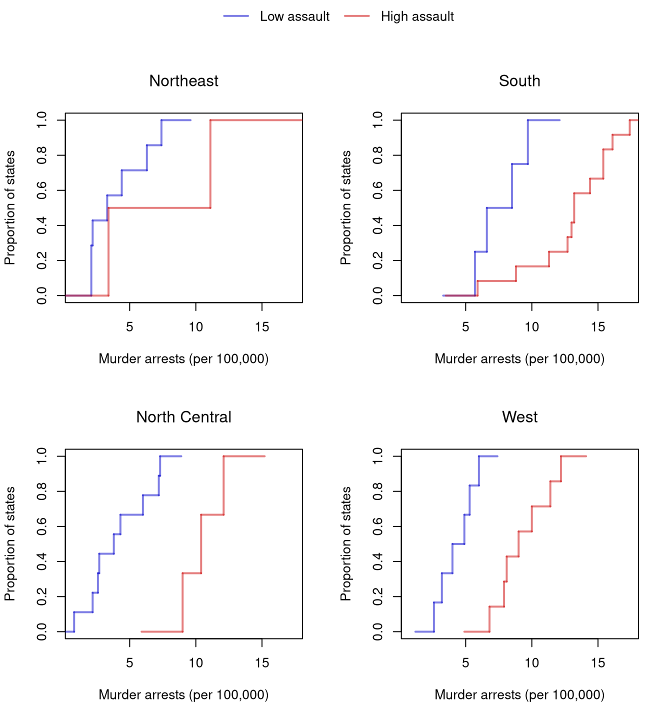
Code
# One panel per region; within each panel, one ECDF for each assault level
col2_high <- rgb(.8, 0, 0, .5)
col2_low  <- rgb(0, 0, .8, .5)
par(mfrow=c(2, 2), oma=c(0, 0, 3, 0))
for (r in levels(xy2_hat$Region)) {
    xy2_r_hat <- xy2_hat[xy2_hat$Region == r, ]
    plot(NULL, xlim=range(xy2_hat$Murder), ylim=c(0, 1),
        xlab='Murder arrests (per 100,000)', ylab='Proportion of states', main=NA)
    F2_lo_hat <- ecdf(xy2_r_hat$Murder[xy2_r_hat$AssaultLevel == 'Low assault'])
    F2_hi_hat <- ecdf(xy2_r_hat$Murder[xy2_r_hat$AssaultLevel == 'High assault'])
    plot(F2_lo_hat, add=TRUE, col=col2_low, lwd=2, verticals=TRUE, do.points=FALSE, col.01line=NA)
    plot(F2_hi_hat, add=TRUE, col=col2_high, lwd=2, verticals=TRUE, do.points=FALSE, col.01line=NA)
    title(r, font.main=1)
}

# One legend for all four panels, drawn on an invisible full-figure overlay
par(fig=c(0, 1, 0, 1), oma=c(0, 0, 0, 0), mar=c(0, 0, 0, 0), new=TRUE)
plot(0, 0, type='n', bty='n', xaxt='n', yaxt='n')
legend('top', horiz=TRUE, bty='n',
    legend=c('Low assault', 'High assault'), col=c(col2_low, col2_high), lwd=2)

Code
# In every region the high-assault curve is to the right of the low-assault curve.
# So the assault-murder link is not an artifact of region.
# The South's high-assault states reach the highest murder rates of any group.
# Its own low-assault states resemble the low-assault states elsewhere.
# The Northeast panel is the thinnest, with only two high-assault states.
# So its curve should be read cautiously.

21.4 Simpson’s Paradox

A relationship visible inside subgroups can flip direction once those subgroups are pooled. The conditional proportions above compare outcomes within values of a third variable \(\hat{z}_{i}\), so we can compare \(\hat{p}(y\mid x,z)\) within each group to the pooled \(\hat{p}(y\mid x)\).

ImportantKey Definition

Simpson’s paradox (Yule 1903; Simpson 1951) arises when a relationship that holds inside all or most subgroups reverses when the data are pooled. The within-group conditional distributions \(\hat{p}(y\mid x, z)\) point one way; the overall \(\hat{p}(y\mid x)\) points the other.

Simpson’s paradox is useful as a warning whenever you are tempted to pool subgroups: the pooled relationship reflects both the within-group pattern and how the subgroups differ in size. The base-rate fallacy is a related composition effect: a category’s share of a pooled statistic can be driven by its size rather than its rate. The Berkeley admissions in Conditional Proportions are the classic example of the paradox. The example is part of a real debate about discrimination (http://homepage.stat.uiowa.edu/~mbognar/1030/Bickel-Berkeley.pdf). A pooled gap can reflect how groups spread across subgroups rather than differences within those subgroups. The same logic applies to the gender pay gap, cross-country growth comparisons, and many other social issues.1 Neither the pooled rates nor the within-group rates alone identify what would happen under an intervention.

A stylized version of the admissions example makes the arithmetic easy to follow. Suppose \(400\) men and \(400\) women apply to one of two departments (English or Engineering). Women can have higher admission rates within both departments yet a lower overall admission rate, if women disproportionately apply to the more selective department (English) and men to the less selective one (Engineering).

School Applicants (Admitted), by Sex and Department
Department Men Women Total
English 100 (40, \(40\%\)) 350 (150, \(43\%\)) 450 (190, \(42\%\))
Engineering 300 (160, \(53\%\)) 50 (30, \(60\%\)) 350 (190, \(54\%\))
Total 400 (200, \(50\%\)) 400 (180, \(45\%\)) 800 (380, \(48\%\))

Using p_dept and p_apply from Conditional Proportions, identify which departments account for most of the reversal, and explain why.

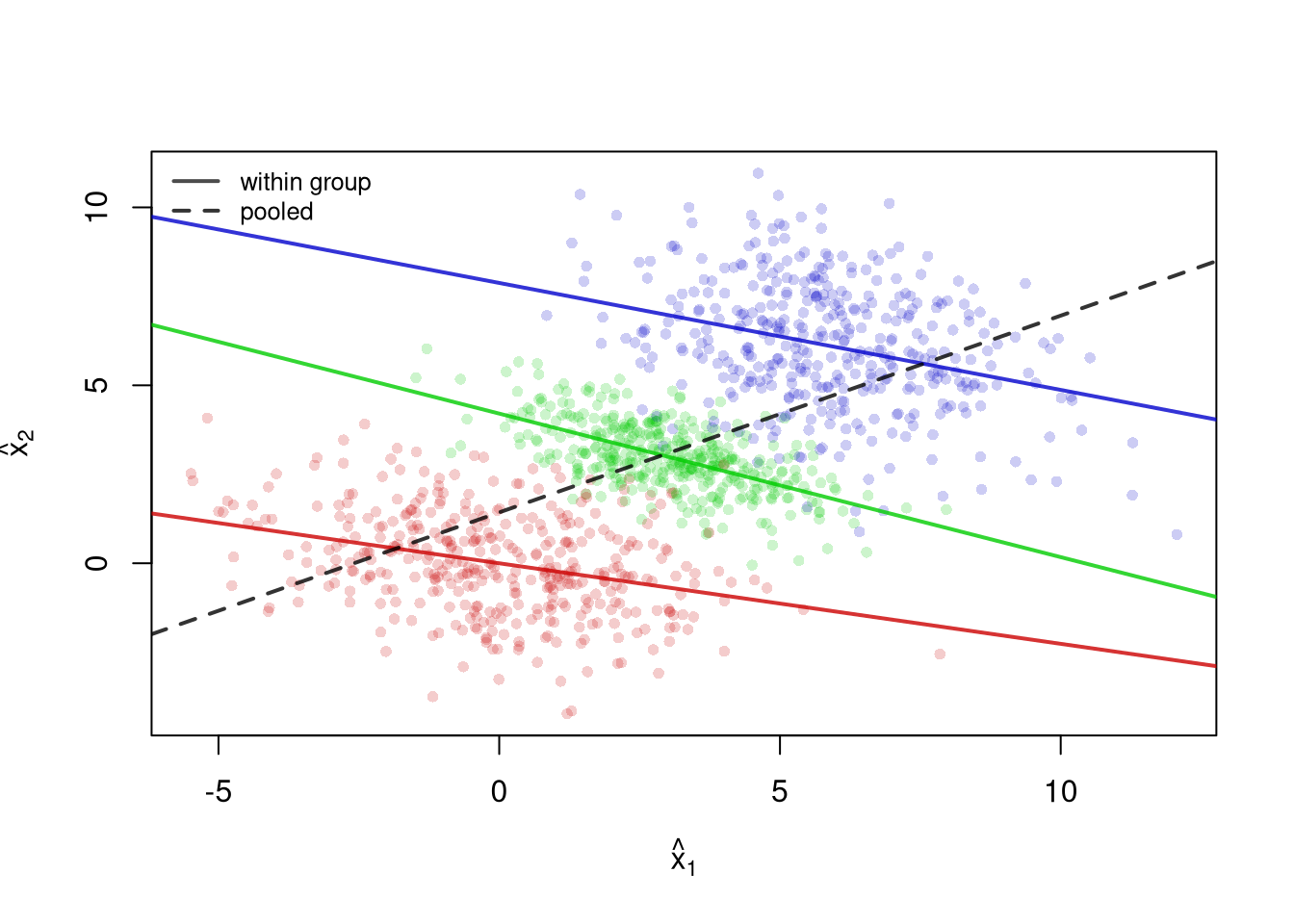
The same issue shows up in continuous data. The figure below shows three simulated groups. Within each group the relationship between \(\hat{x}_{1}\) and \(\hat{x}_{2}\) is negative, but the group centers rise together from lower-left to upper-right.

Each within-group regression line (solid) slopes downward, yet the pooled regression line (dashed) slopes upward. A researcher who ignored the groups would report a positive relationship that holds within no single group. The Simple Regression chapter explains how these lines are fit.

21.5 Exercises

  1. Comment the script you wrote for this chapter, then restart R and check that it runs from a clean session, then check the script with AI as explained in Working with AI. Write three sentences from memory on the main statistical idea of this chapter, and ask the assistant what is wrong, vague, or missing. Finish with your own questions about whatever you found hardest.

  2. Using UCBAdmissions, compute the number of applicants and the admission rate for each department, pooling genders. Then compute the share of all female applicants and the share of all male applicants who applied to each department. Write two sentences that explain the pooled gender gap in admission rates using only these two tables.

  3. The built-in LifeCycleSavings data record five variables for fifty countries, averaged over 1960 to 1970. They are the savings rate sr, the share of the population under 15 (pop15) and over 75 (pop75), real disposable income dpi, and its growth rate ddpi. Draw a scatterplot matrix. Which pair of variables is most tightly related, which panels show a bend rather than a straight cloud, and which country is an outlier in ddpi?

  4. Attach state.region to USArrests and make a conditioning plot of Rape against UrbanPop with one panel per region, on common axes. Then draw the pooled scatterplot. Describe one within-region pattern that the pooled figure hides, or explain why the pooled figure is a fair summary in this case.

  5. Use UCBAdmissions to compute what the pooled admission rate for men and for women would be if both applied to the six departments in the same proportions as all applicants combined. To do this, weight each group’s within-department admission rates by the combined share of applicants in each department. Compare these adjusted rates with the pooled rates shown in this chapter, then explain why the adjustment does not by itself establish whether admissions were discriminatory.

Further Reading

Recall

This chapter described data with three or more variables without fitting a model. Three-way tables and prop.table() with a margin= argument showed that men were admitted to Berkeley at a higher rate than women when departments were pooled. Yet women were admitted at a similar or higher rate within most departments, and the pooled gap mostly reflected women applying to the more selective departments. This reversal is Simpson’s paradox, and a simulated example showed that it can happen with continuous data too. Scatterplot matrices and extra point channels described continuous data. Conditioning plots, grouped boxplots, and ECDFs did it for mixed data. The panels by schooling group showed a pattern that the pooled scatterplot hid. Among workers with exactly \(12\) years of schooling, the mean wage rose from about \(5\) to about \(6\) dollars with experience. Crossing schooling group with sex showed higher wages for men than for women inside every schooling group.

Simpson, E. H. 1951. “The Interpretation of Interaction in Contingency Tables.” Journal of the Royal Statistical Society: Series B (Methodological) 13 (2): 238–41. https://doi.org/10.1111/j.2517-6161.1951.tb00088.x.
Tukey, John Wilder. 1977. Exploratory Data Analysis. Vol. 2. Springer.
Yule, G. Udny. 1903. “Notes on the Theory of Association of Attributes in Statistics.” Biometrika 2 (2): 121–34. https://doi.org/10.1093/biomet/2.2.121.

  1. A ratio can also change due to changes in either the numerator or the denominator.↩︎