The previous chapters summarized bivariate data that we observed. Just as a single random variable has a theoretical mean and variance, a pair \((X_{i}, Y_{i})\) has a theoretical covariance, correlation, and regression coefficient.
This chapter asks three questions.
- What do bivariate sample statistics estimate?
- Joint, marginal, and conditional distributions: these are the theoretical versions of the tables from Bivariate Distributions, with probabilities in place of proportions.
- Conditional expectation: this new object, \(\mathbb{E}[Y_{i}\mid X_{i}=x]\), is the population target for regression.
- Covariance, correlation, and regression coefficient: these are the population counterparts of the sample covariance and correlation and the sample slope. In a linear data generating process, the population slope is \(\beta_{1}=\mathbb{C}[X_{i}, Y_{i}]/\mathbb{V}[X_{i}]\).
- How often does a test give the wrong answer?
- Type I error rate and statistical power: these are the chances of a false positive and of detecting a true effect. Both reuse the permutation test on repeated samples.
- What should we believe after seeing a test result?
- Bayes’ theorem: this reverses the direction of conditioning, which turns a prior belief and a test result into an updated belief. It applies the event version to random variables.
Theoretical Distributions
To talk about what sample statistics estimate, we need a theoretical counterpart to the bivariate observations of the previous chapters.
A random vector \((X_{i}, Y_{i})\) is a pair of random variables drawn together. It is the population analog of one paired observation \((\hat{x}_{i}, \hat{y}_{i})\), described before the data exist.
The random vector is useful as the formal object that the empirical pair \((\hat{x}_{i}, \hat{y}_{i})\) samples from. For example, if we are going to flip two coins, then \((X_{i}, Y_{i})\) corresponds to the unflipped coins and \((\hat{x}_{i}, \hat{y}_{i})\) to the concrete outcomes once they are flipped. Each sample-level object from earlier chapters (\(\hat{p}(x,y)\), \(\hat{c}_{XY}\), \(\hat{r}_{XY}\), \(\hat{b}_{1}\)) has a population counterpart defined at the level of the random vector.
Definitions for Discrete Data
For discrete random variables, the starting point is the table of probabilities for every possible pair of values.
The joint probability of two discrete random variables is the probability that both events \(X_{i}=x\) and \(Y_{i}=y\) occur: \[\text{Prob}(X_{i} = x, Y_{i} = y).\] The joint distribution is the table of these probabilities over all pairs \((x, y)\), summing to one.
The joint probability is useful as the theoretical version of the empirical joint distribution \(\hat{p}(x,y)\) from Bivariate Distributions: the same table structure, but with population probabilities in place of sample proportions. With enough draws, \(\hat{p}(x,y)\) approaches the joint distribution.
A particularly simple special case is when the two variables carry no information about each other.
Two random variables are statistically independent when the joint probability factors as the product of the marginals: \[\text{Prob}(X_{i}=x, Y_{i}=y)=\text{Prob}(X_{i}=x)\text{Prob}(Y_{i}=y) \quad \text{for every } (x, y).\] Equivalently, knowing \(Y_{i}\) tells you nothing about the distribution of \(X_{i}\).
Independence is useful as the cleanest baseline against which to compare real data: most of the dependence statistics in Statistics of Association take value zero when the variables are independent. Independence is sometimes assumed for mathematical simplicity, not because it generally fits data well.
The marginal distributions are then defined as \[\begin{aligned}
\text{Prob}(X_{i} = x) &= \sum_{y} \text{Prob}(X_{i} = x \mid Y_{i} = y) \text{Prob}( Y_{i} = y ) \\
\text{Prob}(Y_{i} = y) &= \sum_{x} \text{Prob}(Y_{i} = y \mid X_{i} = x) \text{Prob}( X_{i} = x ),
\end{aligned}\] which is also known as the law of total probability.
The conditional distributions are defined as \[\begin{aligned}
\text{Prob}(X_{i} = x \mid Y_{i} = y) &= \frac{ \text{Prob}(X_{i} = x, Y_{i} = y)}{ \text{Prob}( Y_{i} = y )} \\
\text{Prob}(Y_{i} = y \mid X_{i} = x) &= \frac{ \text{Prob}(X_{i} = x, Y_{i} = y)}{ \text{Prob}( X_{i} = x )}
\end{aligned}\]
Coin Flips Example
For one example, consider flipping two coins, where we mark whether “heads” is face up with a \(1\) and “tail” with a \(0\). E.g., the first coin has a value of \(x=1\) if it shows heads and \(x=0\) if it shows tails. This table shows both the joint distribution and also each marginal distribution.
Joint and Marginal Distributions of Two Coins
| \(y=0\) |
\(\text{Prob}(X_{i}=0,Y_{i}=0)\) |
\(\text{Prob}(X_{i}=1,Y_{i}=0)\) |
\(\text{Prob}(Y_{i}=0)\) |
| \(y=1\) |
\(\text{Prob}(X_{i}=0,Y_{i}=1)\) |
\(\text{Prob}(X_{i}=1,Y_{i}=1)\) |
\(\text{Prob}(Y_{i}=1)\) |
| Marginal |
\(\text{Prob}(X_{i}=0)\) |
\(\text{Prob}(X_{i}=1)\) |
\(1\) |
Note that different joint distributions can have the same marginal distributions.
Suppose both coins are “fair”: \(\text{Prob}(X_{i}=1)= 1/2\) and \(\text{Prob}(Y_{i}=1\mid X_{i}=x)=1/2\) for either \(x=1\) or \(x=0\), then the four potential outcomes have equal probabilities. \[\begin{aligned}
\text{Prob}(X_{i} = 0, Y_{i} = 0) &= 1/2 \times 1/2 = 1/4 \\
\text{Prob}(X_{i} = 0, Y_{i} = 1) &= 1/4 \\
\text{Prob}(X_{i} = 1, Y_{i} = 0) &= 1/4 \\
\text{Prob}(X_{i} = 1, Y_{i} = 1) &= 1/4 .
\end{aligned}\] The joint distribution is written generally as \[\begin{aligned}
\text{Prob}(X_{i} = x, Y_{i} = y) &= \text{Prob}(X_{i} = x) \text{Prob}(Y_{i} = y).
\end{aligned}\]
Code
# Create a 2x2 matrix for the joint distribution.
# Rows correspond to X (coin 1), and columns correspond to Y (coin 2).
probs <- c(0.25, 0.25, 0.25, 0.25) # Fair coin
P_xy <- matrix( probs, nrow = 2, ncol = 2)
rownames(P_xy) <- c('Y=0', 'Y=1')
colnames(P_xy) <- c('X=0', 'X=1')
P_xy
##      X=0  X=1
## Y=0 0.25 0.25
## Y=1 0.25 0.25

# Draw N bivariate observations
N <- 500
xy_vals <- expand.grid(y = 0:1, x = 0:1)
draws <- sample(nrow(xy_vals), N, replace = TRUE, prob = P_xy)
x_sim <- xy_vals[draws, 'x']
y_sim <- xy_vals[draws, 'y']

# With enough draws, empirical frequencies approach the true probabilities
table(y_sim, x_sim) / N
##      x_sim
## y_sim     0     1
##     0 0.242 0.298
##     1 0.242 0.218
P_xy
##      X=0  X=1
## Y=0 0.25 0.25
## Y=1 0.25 0.25
The marginal distribution of the second coin is \[\begin{aligned}
\text{Prob}(Y_{i} = 0) &= \text{Prob}(Y_{i} = 0 \mid X_{i} = 0) \text{Prob}(X_{i}=0) + \text{Prob}(Y_{i} = 0 \mid X_{i} = 1) \text{Prob}(X_{i}=1) \\
&= 1/2 (1/2) + 1/2 (1/2) = 1/2 \\
\text{Prob}(Y_{i} = 1) &= \text{Prob}(Y_{i} = 1 \mid X_{i} = 0) \text{Prob}(X_{i}=0) + \text{Prob}(Y_{i} = 1 \mid X_{i} = 1) \text{Prob}(X_{i}=1) \\
&= 1/2 (1/2) + 1/2 (1/2) = 1/2
\end{aligned}\]
The marginal distribution of the first coin is found in the exact same way \[\begin{aligned}
\text{Prob}(X_{i} = 0) &= \text{Prob}(X_{i} = 0 \mid Y_{i} = 0) \text{Prob}(Y_{i}=0) + \text{Prob}(X_{i} = 0 \mid Y_{i} = 1) \text{Prob}(Y_{i}=1) \\
&= 1/2 (1/2) + 1/2 (1/2) = 1/2 \\
\text{Prob}(X_{i} = 1) &= \text{Prob}(X_{i} = 1 \mid Y_{i} = 0) \text{Prob}(Y_{i}=0) + \text{Prob}(X_{i} = 1 \mid Y_{i} = 1) \text{Prob}(Y_{i}=1) \\
&= 1/2 (1/2) + 1/2 (1/2) = 1/2
\end{aligned}\]
Altogether, we find
Two Fair Coins
| \(y=0\) |
\(1/4\) |
\(1/4\) |
\(1/2\) |
| \(y=1\) |
\(1/4\) |
\(1/4\) |
\(1/2\) |
| Marginal |
\(1/2\) |
\(1/2\) |
\(1\) |
Code
# Compute the marginal distributions.
# Marginal for X: sum across columns.
P_x <- colSums(P_xy)
P_x
## X=0 X=1
## 0.5 0.5
# Marginal for Y: sum across rows.
P_y <- rowSums(P_xy)
P_y
## Y=0 Y=1
## 0.5 0.5

# Compute the conditional probabilities Prob(Y | X).
PY_x <- matrix(0, nrow = 2, ncol = 2)
for (j in c(1, 2)) {
  PY_x[, j] <- P_xy[, j] / P_x[j]
}
rownames(PY_x) <- c('Y=0', 'Y=1')
colnames(PY_x) <- c('given X=0', 'given X=1')
PY_x
##     given X=0 given X=1
## Y=0       0.5       0.5
## Y=1       0.5       0.5
Are the coins statistically independent?
Now consider a second example, where the second coin is “Completely Unfair”, so that it is always the same as the first. The outcomes generated with a Completely Unfair coin are the same as if we only flipped one coin. \[\begin{aligned}
\text{Prob}(X_{i} = 0, Y_{i} = 0) &= 1/2 \\
\text{Prob}(X_{i} = 0, Y_{i} = 1) &= 0 \\
\text{Prob}(X_{i} = 1, Y_{i} = 0) &= 0 \\
\text{Prob}(X_{i} = 1, Y_{i} = 1) &= 1/2 .
\end{aligned}\] The joint distribution is written generally as \[\begin{aligned}
\text{Prob}(X_{i} = x, Y_{i} = y) &= \text{Prob}(X_{i} = x) \mathbf{1}( x=y ),
\end{aligned}\] where \(\mathbf{1}(x=y)\) equals \(1\) when \(x=y\) and \(0\) otherwise. The marginal distribution of the second coin is \[\begin{aligned}
\text{Prob}(Y_{i} = 0)
&= \text{Prob}(Y_{i} = 0 \mid X_{i} = 0) \text{Prob}(X_{i}=0) + \text{Prob}(Y_{i} = 0 \mid X_{i} = 1) \text{Prob}(X_{i} = 1) \\
&= 1 (1/2) + 0(1/2) = 1/2 . \\
\text{Prob}(Y_{i} = 1)
&= \text{Prob}(Y_{i} = 1 \mid X_{i} =0) \text{Prob}( X_{i} = 0) + \text{Prob}(Y_{i} = 1 \mid X_{i} = 1) \text{Prob}( X_{i} = 1) \\
&= 0 (1/2) + 1 (1/2) = 1/2 .
\end{aligned}\] which is the same marginal as in the first example!
The marginal distribution of the first coin is found in the exact same way (show this yourself).
Altogether, we find
A Fair Coin and a Completely Unfair Coin
| \(y=0\) |
\(1/2\) |
\(0\) |
\(1/2\) |
| \(y=1\) |
\(0\) |
\(1/2\) |
\(1/2\) |
| Marginal |
\(1/2\) |
\(1/2\) |
\(1\) |
Code
# Create the joint distribution matrix for the unfair coin case.
probs <- c(0.5, 0, 0, 0.5) # unfair coin

P_xy <- matrix( probs, nrow = 2, ncol = 2)
rownames(P_xy) <- c('Y=0', 'Y=1')
colnames(P_xy) <- c('X=0', 'X=1')
P_xy
##     X=0 X=1
## Y=0 0.5 0.0
## Y=1 0.0 0.5


# Compute the marginal distributions.
# Marginal for X: sum across columns.
P_x <- colSums(P_xy)
P_x
## X=0 X=1
## 0.5 0.5
# Marginal for Y: sum across rows.
P_y <- rowSums(P_xy)
P_y
## Y=0 Y=1
## 0.5 0.5

# Compute the conditional probabilities Prob(Y | X).
PY_x <- matrix(0, nrow = 2, ncol = 2)
for (j in c(1, 2)) {
  PY_x[, j] <- P_xy[, j] / P_x[j]
}
rownames(PY_x) <- c('Y=0', 'Y=1')
colnames(PY_x) <- c('given X=0', 'given X=1')
PY_x
##     given X=0 given X=1
## Y=0         1         0
## Y=1         0         1
Are the coins statistically independent?
Try computing conditional probabilities for another unfair set of coins below. Explain why the marginal distribution of the second coin is balanced.
Code
probs <- c(0.4, 0.2, 0.1, 0.3)
P_xy <- matrix(probs, nrow = 2,
  dimnames = list(c('Y=0', 'Y=1'), c('X=0', 'X=1')))

# Draw N bivariate observations
xy_vals <- expand.grid(y = 0:1, x = 0:1)
N <- 500
draws <- sample(nrow(xy_vals), N, replace = TRUE, prob = P_xy)
x_sim <- xy_vals[draws, 'x']
y_sim <- xy_vals[draws, 'y']

table(y_sim, x_sim) / N
##      x_sim
## y_sim     0     1
##     0 0.398 0.116
##     1 0.202 0.284
P_xy
##     X=0 X=1
## Y=0 0.4 0.1
## Y=1 0.2 0.3
Sometimes we observe one variable and want to learn about the other, which reverses the direction of conditioning.
Bayes’ theorem (Bayes 1763) relates the two conditional directions: \[\text{Prob}(X_{i}=x \mid Y_{i}=y) = \frac{\text{Prob}(Y_{i}=y \mid X_{i}=x)\,\text{Prob}(X_{i}=x)}{\text{Prob}(Y_{i}=y)}.\]
Bayes’ theorem is useful because it is exactly how an observation updates a prior belief. It applies the event version of Bayes’ theorem to random variables. Building on the coin-flip examples above, suppose we observe the outcome of the second coin (\(Y_{i}\)) and want to update our belief about the first coin (\(X_{i}\)).
Unfair coins. Now consider the joint distribution from the Test Yourself above, with probs <- c(0.4, 0.2, 0.1, 0.3):
Two Unfair Coins
| \(y=0\) |
\(0.4\) |
\(0.1\) |
\(0.5\) |
| \(y=1\) |
\(0.2\) |
\(0.3\) |
\(0.5\) |
| Marginal |
\(0.6\) |
\(0.4\) |
\(1\) |
The prior is \(\text{Prob}(X_{i}=1)=0.4\). The conditional probabilities of heads on the second coin are \[
\text{Prob}(Y_{i}=1\mid X_{i}=1) = \frac{0.3}{0.4} = 0.75,\quad
\text{Prob}(Y_{i}=1\mid X_{i}=0) = \frac{0.2}{0.6} = \frac{1}{3}.
\] Applying Bayes’ theorem, \[\begin{aligned}
\text{Prob}(X_{i}=1\mid Y_{i}=1)
&= \frac{0.75 \times 0.4}{0.75 \times 0.4 + \frac{1}{3}\times 0.6}
= \frac{0.3}{0.3+0.2} = 0.6.
\end{aligned}\] The prior probability of heads on the first coin was \(0.4\), but after seeing heads on the second coin, it increases to \(0.6\). The coins are not independent: when the second coin shows heads, it is more likely that the first coin also shows heads.
Code
# Unfair coins
probs <- c(0.4, 0.2, 0.1, 0.3)
P_xy <- matrix(probs, nrow = 2,
  dimnames = list(c('Y=0', 'Y=1'), c('X=0', 'X=1')))
P_xy
##     X=0 X=1
## Y=0 0.4 0.1
## Y=1 0.2 0.3

# Marginals
P_x <- colSums(P_xy)
P_y <- rowSums(P_xy)

# Prob(Y=1 | X=x)
PY1_x <- P_xy['Y=1', ] / P_x
PY1_x
##       X=0       X=1
## 0.3333333 0.7500000

# Posterior: Prob(X=1 | Y=1)
posterior_x1 <- (PY1_x['X=1'] * P_x['X=1']) / P_y['Y=1']
posterior_x1  # prior was 0.4, posterior is 0.6
## X=1
## 0.6

# Also compute Prob(X=1 | Y=0)
PY0_x <- P_xy['Y=0', ] / P_x
posterior_x1_y0 <- (PY0_x['X=1'] * P_x['X=1']) / P_y['Y=0']
posterior_x1_y0  # seeing tails lowers belief to 0.2
## X=1
## 0.2
Are the coins statistically independent?
Definitions for Continuous Data
The joint distribution is defined as \[\begin{aligned}
F(x, y) &= \text{Prob}(X_{i} \leq x, Y_{i} \leq y)
\end{aligned}\] The marginal distributions are then defined as \[\begin{aligned}
F_{X}(x) &= F(x, \infty) \\
F_{Y}(y) &= F(\infty, y).
\end{aligned}\] which is called marginalizing (an application of the law of total probability). Variables are statistically independent if \(F(x, y) = F_{X}(x)F_{Y}(y)\) for all \(x, y\).
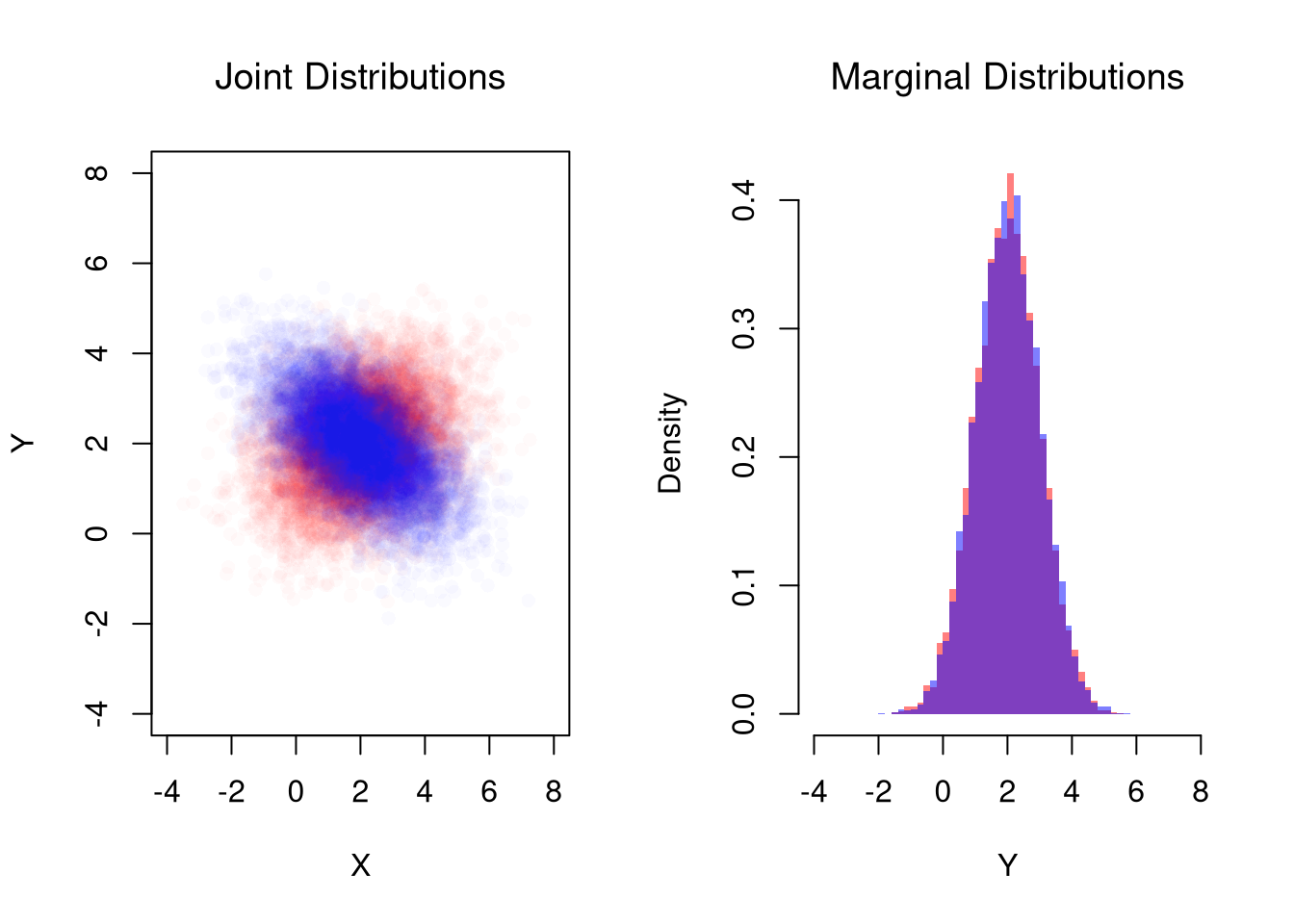
The most-used parametric joint distribution on continuous data is the bivariate analog of the Normal.
A bivariate normal distribution describes a random vector \((X_{i}, Y_{i})\) whose joint density is the multivariate normal with mean vector \((\mathbb{E}[X_{i}], \mathbb{E}[Y_{i}])\), variances \((\mathbb{V}[X_{i}], \mathbb{V}[Y_{i}])\), and correlation \(\rho\).
The bivariate normal is useful for analytical work on multivariate random variables. Both marginals are normal, and every conditional \(Y_{i} \mid X_{i} = x\) is also normal with a linear conditional mean. Many results for one Normal random variable therefore extend to the pair.
Code
library('mvtnorm')

# Simulate Bivariate Data
N <- 10000
Mu <- c(2, 2) ## Means

Sigma1 <- matrix(c(2, -.8, -.8, 1), 2, 2) ## CoVariance Matrix 1
xy1_sim <- rmvnorm(N, Mu, Sigma1)
colnames(xy1_sim) <- c('x_sim', 'y_sim')

Sigma2 <- matrix(c(2, .4, .4, 1), 2, 2) ## CoVariance Matrix 2
xy2_sim <- rmvnorm(N, Mu, Sigma2)
colnames(xy2_sim) <- c('x_sim', 'y_sim')

par(mfrow=c(1, 2))
## Different diagonals
plot(xy2_sim, col=rgb(1, 0, 0, 0.02), pch=16,
    main=NA,
    ylim=c(-4, 8), xlim=c(-4, 8),
    xlab='X', ylab='Y')
title('Joint Distributions', font.main=1)
points(xy1_sim, col=rgb(0, 0, 1, 0.02), pch=16)
## Same marginal distributions
xbks <- seq(-4, 8, by=.2)
hist(xy2_sim[, 2], col=rgb(1, 0, 0, 0.5),
    breaks=xbks, border=NA, freq=FALSE,
    xlab='Y',
    main=NA)
title('Marginal Distributions', font.main=1)
hist(xy1_sim[, 2], col=rgb(0, 0, 1, 0.5),
    add=TRUE, breaks=xbks, border=NA, freq=FALSE)
Independent normal random variables are a special case of the bivariate normal. With both variances equal to \(1\) and \(\rho=0\), drawing \(X_{i}\) and \(Y_{i}\) separately gives the same joint distribution as one draw from the bivariate normal.
Code
# Two independent standard normal random variables
n <- 2e4
xy_iid_sim <- cbind(rnorm(n), rnorm(n))

# One joint draw from a bivariate normal with zero correlation
xy_joint_sim <- mvtnorm::rmvnorm(n, c(0, 0))

par(mfrow=c(1, 2))
plot(xy_iid_sim, col=grey(0, .05), pch=16,
    xlim=c(-5, 5), ylim=c(-5, 5),
    main=NA, xlab='X', ylab='Y')
title('Two Independent Draws', font.main=1)
plot(xy_joint_sim, col=grey(0, .05), pch=16,
    xlim=c(-5, 5), ylim=c(-5, 5),
    main=NA, xlab='X', ylab='Y')
title('One Joint Draw', font.main=1)
Code
# The joint density equals the product of the two marginal densities
d1 <- dnorm(xy_iid_sim[, 1])*dnorm(xy_iid_sim[, 2])
d2 <- mvtnorm::dmvnorm(xy_iid_sim, c(0, 0))
head(cbind(product=d1, joint=d2))
##         product      joint
## [1,] 0.04924204 0.04924204
## [2,] 0.07451359 0.07451359
## [3,] 0.14921940 0.14921940
## [4,] 0.06446184 0.06446184
## [5,] 0.03244693 0.03244693
## [6,] 0.15220066 0.15220066
Other joint distributions exist; see e.g., https://cran.r-project.org/web/packages/NonNorMvtDist/NonNorMvtDist.pdf.
Statistics
Conditional Expectation
The natural population object that regression tries to estimate is the average of \(Y_{i}\) within each subpopulation defined by \(X_{i}\).
The conditional expectation \(\mathbb{E}[Y_{i}\mid X_{i}=x]\) is the population mean of \(Y_{i}\) inside the subpopulation where \(X_{i}=x\): \[\mathbb{E}[Y_{i}\mid X_{i}=x]=\sum_{y} y\,\text{Prob}(Y_{i}=y\mid X_{i}=x).\]
The conditional expectation is useful as the population target for regression. The sample conditional means \(\hat{m}_{Y}(x)\) from Two Groups estimate \(\mathbb{E}[Y_{i}\mid X_{i}=x]\). The fitted line from Simple Regression estimates its best linear approximation. The formula above sums over conditional probabilities for discrete \(X_{i}\); for continuous \(X_{i}\) the conditional expectation function traces a smooth curve indexed by \(x\) (the integral version replaces the sum).
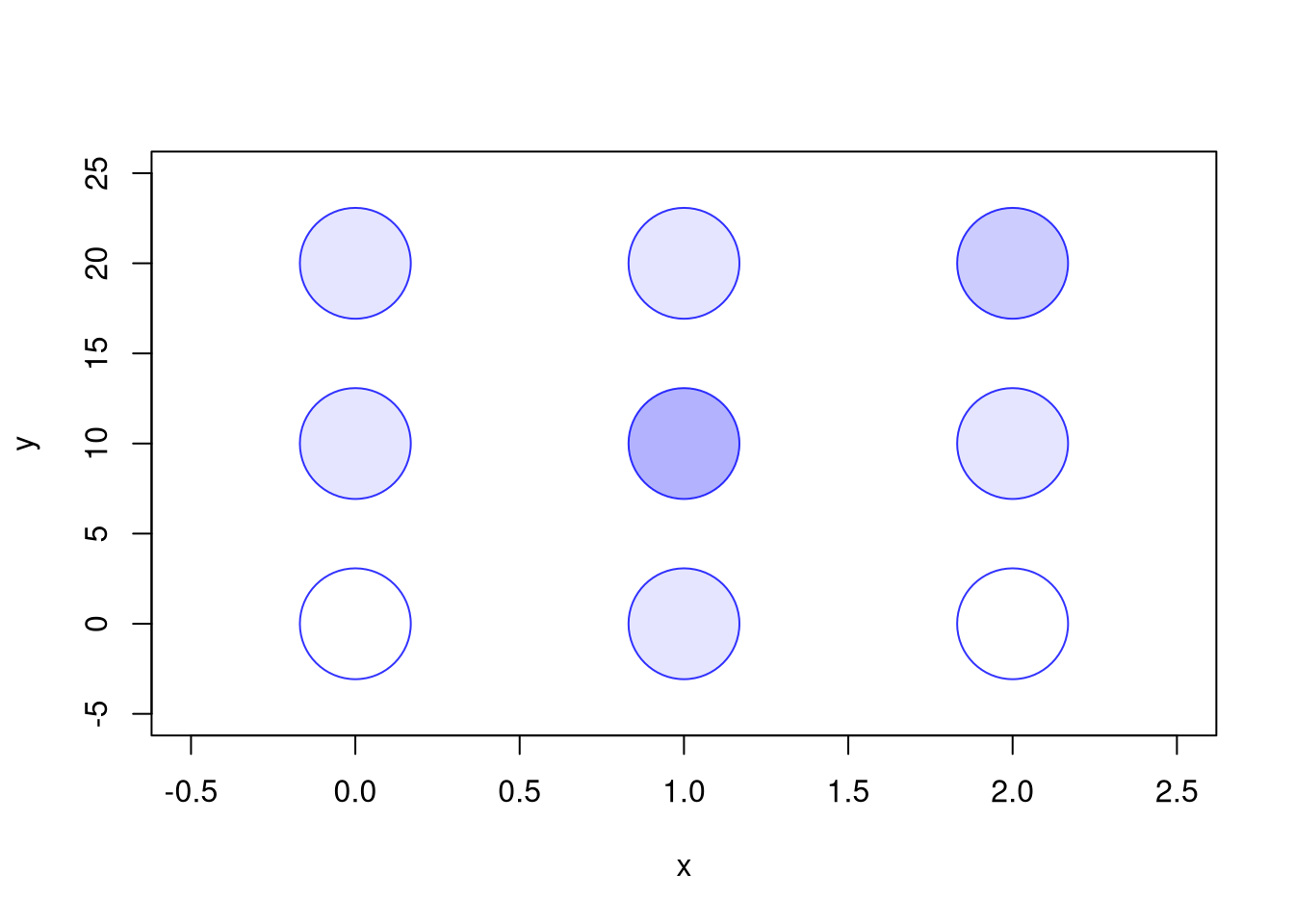
For example, consider a bivariate random vector with three outcomes for \(X_{i}\) and three outcomes for \(Y_{i}\).
Joint Distribution with Three Outcomes Each
| \(y=0\) |
\(0.0\) |
\(0.1\) |
\(0.0\) |
| \(y=10\) |
\(0.1\) |
\(0.3\) |
\(0.1\) |
| \(y=20\) |
\(0.1\) |
\(0.1\) |
\(0.2\) |
The plot below shows each outcome \((x,y)\) with deeper colors reflecting higher probability events.
Code
## MAIN EXAMPLE
# Make a Probability Table
x <- c(0, 1, 2)
y <- c(0, 10, 20)
P_xy <- matrix(c(
    0.0, 0.1, 0.0,
    0.1, 0.3, 0.1,
    0.1, 0.1, 0.2
), nrow=3, ncol=3, byrow=TRUE)
rownames(P_xy) <- paste0('y=', y)
colnames(P_xy) <-  paste0('x=', x)
P_xy
##      x=0 x=1 x=2
## y=0  0.0 0.1 0.0
## y=10 0.1 0.3 0.1
## y=20 0.1 0.1 0.2

# Plot joint distribution
prob_table <- expand.grid(x=x, y=y)
prob_table[, 'probabilities'] <- as.vector(t(P_xy))
plot(prob_table[, 'x'], prob_table[, 'y'],
     xlim=c(-0.5, 2.5), ylim=c(-5, 25),
     pch=21, cex=8, col=rgb(0, 0, 1, .8),
     bg=rgb(0, 0, 1, prob_table[, 'probabilities']),
     main=NA, xlab='x', ylab='y')
We can compute marginals from the table, \[\begin{aligned}
\text{Prob}(X_{i}=0)=0.2,\quad & \text{Prob}(X_{i}=1)=0.5 ,\quad \text{Prob}(X_{i}=2) = 0.3 \\
\text{Prob}(Y_{i}=0)=0.1,\quad & \text{Prob}(Y_{i}=10)=0.5 ,\quad \text{Prob}(Y_{i}=20) = 0.4
\end{aligned}\]
This gives us conditional probabilities and hence also conditional expectations; \[\begin{aligned}
\mathbb{E}[Y_{i}\mid X_{i}=0] &= 0\frac{0}{0.2} + 10\frac{0.1}{0.2} + 20\frac{0.1}{0.2} = 0 + \frac{10}{2} + \frac{20}{2} = 15, \\
\mathbb{E}[Y_{i}\mid X_{i}=1] &= 0\frac{0.1}{0.5} + 10\frac{0.3}{0.5} + 20\frac{0.1}{0.5} = 0 + \frac{30}{5} + \frac{20}{5} = 10, \\
\mathbb{E}[Y_{i}\mid X_{i}=2] &= 0\frac{0}{0.3} + 10\frac{0.1}{0.3} + 20\frac{0.2}{0.3} = 0 + \frac{10}{3} + \frac{40}{3} = \frac{50}{3} \approx 16.67.
\end{aligned}\] Note that the conditional mean is non-monotonic: \[\begin{aligned}
\frac{\mathbb{E}[Y_{i}\mid X_{i}=1] - \mathbb{E}[Y_{i}\mid X_{i}=0]}{1-0} &= \frac{10 - 15}{1} = -5, \\
\frac{\mathbb{E}[Y_{i}\mid X_{i}=2] - \mathbb{E}[Y_{i}\mid X_{i}=1]}{2-1} &= \frac{\frac{50}{3} - 10}{1} = \frac{20}{3} \approx 6.67.
\end{aligned}\] It decreases from \(x=0\) to \(x=1\) and then increases from \(x=1\) to \(x=2\).
Code
## MAIN EXAMPLE
# Compute Marginals
P_x <- colSums(P_xy) #Prob(X_i=x)
P_y <- rowSums(P_xy) #Prob(Y_i=y)

# Compute the conditional probabilities Prob(Y_i=y | X_i=x).
PY_x <- matrix(0, nrow = 3, ncol = 3)
for (j in seq(ncol(P_xy)) ) {
  PY_x[, j] <- P_xy[, j] / P_x[j]
}
rownames(PY_x) <- paste0('Y=', y)
colnames(PY_x) <- paste0('given X=', x)
PY_x
##      given X=0 given X=1 given X=2
## Y=0        0.0       0.2 0.0000000
## Y=10       0.5       0.6 0.3333333
## Y=20       0.5       0.2 0.6666667

# Computational Shortcut: PY_x <- t( t(P_xy) / P_x )

# Conditional expectation E[Y_i|X_i=x]
EY_x <- colSums(PY_x * y)
EY_x
## given X=0 given X=1 given X=2
##  15.00000  10.00000  16.66667

# Contrast with Grand Means
EX <- sum(x * P_x)
EY <- sum(y * P_y)
EY
## [1] 13

# E[X_i|Y_i=y]
# PX_y <- P_xy / P_y  #Prob(X_i=x | Y_i=y)
# EX_y <- PX_y %*% x
Covariance
We can also dig a little deeper into the other bivariate statistics we compute. When we know how the data are generated, we can often compute the foundational covariance statistic. The covariance is the expected product of deviations from the population means: \[\begin{aligned}
\mathbb{C}[X_{i}, Y_{i}]
&= \mathbb{E}\left[(X_{i} - \mathbb{E}[X_{i}])(Y_{i} - \mathbb{E}[Y_{i}])\right] \\
&= \sum_{x}\sum_{y} (x - \mathbb{E}[X_{i}])(y - \mathbb{E}[Y_{i}]) \text{Prob}(X_{i} = x, Y_{i} = y)
\end{aligned}\]
Using the marginal distributions from before allows us to compute the means: \[\begin{aligned}
\mathbb{E}[X_{i}] &= 0(0.2)+1(0.5)+2(0.3) = 1.1 \\
\mathbb{E}[Y_{i}] &= 0(0.1)+10(0.5)+20(0.4) = 13
\end{aligned}\] We can then compute the cell-by-cell contributions: \(\text{Prob}(X_{i} = x, Y_{i} = y) (x-\mathbb{E}[X_{i}])(y-\mathbb{E}[Y_{i}])\), which plug in to the covariance formula; \[
\begin{array}{l l r r r r r}
\hline
x & y & \text{Prob}(X_{i}=x, Y_{i}=y) & x-\mathbb{E}[X_{i}] & y-\mathbb{E}[Y_{i}] & (x-\mathbb{E}[X_{i}])(y-\mathbb{E}[Y_{i}]) & \text{Contribution}\\
\hline
0 & 0 & 0.0 & -1.1 & -13 & 14.3 & 0\\
0 & 10 & 0.1 & -1.1 & -3 & 3.3 & 0.330\\
0 & 20 & 0.1 & -1.1 & 7 & -7.7 & -0.770\\
1 & 0 & 0.1 & -0.1 & -13 & 1.3 & 0.130\\
1 & 10 & 0.3 & -0.1 & -3 & 0.3 & 0.090\\
1 & 20 & 0.1 & -0.1 & 7 & -0.7 & -0.070\\
2 & 0 & 0.0 & 0.9 & -13 & -11.7 & 0\\
2 & 10 & 0.1 & 0.9 & -3 & -2.7 & -0.270\\
2 & 20 & 0.2 & 0.9 & 7 & 6.3 & 1.260\\
\hline
\end{array}
\] \[\begin{aligned}
\mathbb{C}[X_{i},Y_{i}] &= \sum_{x} \sum_{y} \left(x-\mathbb{E}[X_{i}]\right)\left(y-\mathbb{E}[Y_{i}]\right) \text{Prob}\left(X_{i} = x, Y_{i} = y\right) \\
&= 0 + 0.330 -0.770 + 0.130 + 0.090 -0.070 +0 -0.270 + 1.260
= 0.7
\end{aligned}\]
Note that you can do the above calculations using the computer instead of by hand.
Code
## MAIN EXAMPLE
# Compute Covariance
dxy_grid <- expand.grid(dy=y-EY, dx=x-EX)[, c(2, 1)]
dxy_grid[, 'p'] <- as.vector(P_xy)
dxy_grid[, 'contribution'] <- dxy_grid[, 'dx'] * dxy_grid[, 'dy'] * dxy_grid[, 'p']
CovXY <- sum(dxy_grid[, 'contribution'])
CovXY
## [1] 0.7
We can now use the covariance to compute the often-used Pearson correlation.
The Pearson correlation (Pearson 1896) divides the covariance by the product of the two standard deviations: \[
\frac{\mathbb{C}[X_{i}, Y_{i}] }{ \sqrt{\mathbb{V}[X_{i}]} \sqrt{\mathbb{V}[Y_{i}]} }
\]
To compute this statistic in the previous example, we first need the variances \[\begin{aligned}
\mathbb{V}[X_{i}] &= \sum_{x} (x-\mathbb{E}[X_{i}])^2 \text{Prob}(X_{i} = x) \\
&= (0-1.1)^2(0.2)+(1-1.1)^2(0.5)+(2-1.1)^2(0.3)=0.49 \\
\mathbb{V}[Y_{i}] &= \sum_{y} (y-\mathbb{E}[Y_{i}])^2 \text{Prob}(Y_{i} = y) \\
&= (0-13)^2(0.1)+(10-13)^2(0.5)+(20-13)^2(0.4)=41
\end{aligned}\] Then we can find the correlation as \[\begin{aligned}
\frac{\mathbb{C}[X_{i},Y_{i}]}{ \sqrt{\mathbb{V}[X_{i}]} \sqrt{\mathbb{V}[Y_{i}]} }
&= \frac{0.7}{\sqrt{0.49} \sqrt{41}} = \frac{0.7}{0.7 \sqrt{41}} = \frac{1}{\sqrt{41}} \approx 0.156,
\end{aligned}\] which suggests a weak positive association between the variables.
Code
## MAIN EXAMPLE
# CovXY defined above
# Compute Variances
VX <- sum( (x-EX)^2 * P_x)
SX <- sqrt(VX)
VY <- sum( (y-EY)^2 * P_y)
SY <- sqrt(VY)

# Compute Correlation
CorXY <- CovXY / (SX * SY)
CorXY
## [1] 0.1561738
Compute the correlation for bivariate data with these probabilities, using both math (first) and the computer (second)
Joint Distribution A
| \(y=0\) |
\(0.05\) |
\(0.20\) |
| \(y=1\) |
\(0.05\) |
\(0.20\) |
| \(y=2\) |
\(0.05\) |
\(0.20\) |
| \(y=3\) |
\(0.05\) |
\(0.20\) |
Also compute the correlation for bivariate data with these probabilities
Joint Distribution B
| \(y=0\) |
\(0.05\) |
\(0.05\) |
| \(y=1\) |
\(0.10\) |
\(0.10\) |
| \(y=2\) |
\(0.15\) |
\(0.15\) |
| \(y=3\) |
\(0.20\) |
\(0.20\) |
Also compute the correlation for bivariate data with these probabilities
Joint Distribution C
| \(y=0\) |
\(0.05\) |
\(0.15\) |
| \(y=1\) |
\(0.05\) |
\(0.15\) |
| \(y=2\) |
\(0.10\) |
\(0.20\) |
| \(y=3\) |
\(0.10\) |
\(0.20\) |
Explain intuitively when the correlation equals \(0\) and when it does not.
Regression Coefficient
Just as the sample slope \(\hat{b}_{1}\) summarized a sample, its population counterpart describes how the data are generated.
A linear data generating process is \[Y_{i} = \beta_{0} + \beta_{1} X_{i} + \epsilon_{i}, \quad \mathbb{E}[\epsilon_{i} \mid X_{i}=x] = 0 \text{ for every } x,\] where the fixed numbers \(\beta_{0}\) and \(\beta_{1}\) are the (theoretical) regression coefficients and \(\epsilon_{i}\) is the population error term. In this model, the slope equals the covariance over the variance of \(X_{i}\): \[\beta_{1} = \frac{\mathbb{C}[X_{i}, Y_{i}] }{ \mathbb{V}[X_{i}] }.\]
To see why, note that the error has mean zero at every \(x\), so it also has mean zero overall, and \(Y_{i} - \mathbb{E}[Y_{i}] = \beta_{1}(X_{i}-\mathbb{E}[X_{i}]) + \epsilon_{i}\). Then \[\begin{aligned}
\mathbb{C}[X_{i}, Y_{i}]
&= \mathbb{E}\left[(X_{i}-\mathbb{E}[X_{i}])\left(\beta_{1}(X_{i}-\mathbb{E}[X_{i}]) + \epsilon_{i}\right)\right] \\
&= \beta_{1}\mathbb{E}\left[(X_{i}-\mathbb{E}[X_{i}])^2\right] + \mathbb{E}\left[(X_{i}-\mathbb{E}[X_{i}])\epsilon_{i}\right] \\
&= \beta_{1}\mathbb{V}[X_{i}],
\end{aligned}\] where the last term is zero because \(\epsilon_{i}\) averages to zero at each value of \(X_{i}\). Dividing both sides by \(\mathbb{V}[X_{i}]\) gives the formula in the definition.
\(\beta_{1}\) is useful as the population target of the sample slope \(\hat{b}_{1} = \hat{c}_{XY}/\hat{v}_{X}\) from Simple Regression: when the data come from a linear data generating process, OLS estimates \(\beta_{1}\) from a finite sample. In that case, the conditional expectation is itself a straight line, \(\mathbb{E}[Y_{i}\mid X_{i}=x] = \beta_{0} + \beta_{1}x\), because the error averages to zero at every \(x\). However, the ratio \(\mathbb{C}[X_{i}, Y_{i}]/\mathbb{V}[X_{i}]\) can be computed for any joint distribution, even when no linear data generating process exists.
For the \(3\times3\) table above, the conditional expectation computed earlier is not a straight line (it falls from \(x=0\) to \(x=1\), then rises), so the data are not generated by a linear model and there is no true \(\beta_{1}\). We already found \(\mathbb{C}[X_{i}, Y_{i}] = 0.7\) and \(\mathbb{V}[X_{i}] = 0.49\), so the ratio is still \[
\frac{\mathbb{C}[X_{i}, Y_{i}]}{\mathbb{V}[X_{i}]} = \frac{0.7}{0.49} = \frac{70}{49} = \frac{10}{7} \approx 1.43.
\] This is the slope of the best straight-line approximation to the conditional expectation. The line is “best” in the sense that it minimizes mean squared error among all linear approximations to the conditional expectation function. OLS estimates this slope from samples of the table, and it is positive because the line captures the overall upward tendency. But when the conditional expectation bends, the best line still misses: here it misses the dip at \(x=1\).
Code
## MAIN EXAMPLE
# CovXY and VX defined above
# Slope of the best linear approximation: covariance over variance of X
CovXY / VX
## [1] 1.428571
Type I and Type II Errors
A hypothesis test starts with a null \(H_{0}\) and an alternative \(H_{A}\), and produces a decision (reject or fail-to-reject) from finite sample data. Because the data have variability, the decision can be wrong in two ways (Neyman and Pearson 1933).
A Type I error is rejecting \(H_{0}\) when \(H_{0}\) is true (a false positive). A Type II error is failing to reject \(H_{0}\) when \(H_{0}\) is false (a false negative).
This distinction is useful because the two error types are managed by different levers: we control Type I error by setting the significance level \(\alpha=\text{Prob}(\text{Type I})\) before looking at the data, while Type II error is harder to control directly and depends on the sample size and the true effect size. Reducing one error rate usually raises the other for a fixed sample.
Type I and Type II Errors
| \(H_{0}\) is True |
Correct (no detection) |
Type I Error (False Positive) |
| \(H_{0}\) is False |
Type II Error (False Negative; missed detection) |
Correct (effect detected) |
Here is a Courtroom example: Someone suspected of committing a crime is at trial, and they are either guilty or not (a Bernoulli random variable). You hypothesize that the suspect is innocent, and a jury can either convict them (decide guilty) or free them (decide not-guilty). Recall that fail-to-reject a hypothesis does not mean accepting it, so deciding not-guilty does not necessarily mean innocent.
Courtroom Decisions
| Suspect Innocent |
Correctly Freed |
Falsely Convicted |
| Suspect Guilty |
Falsely Freed |
Correctly Convicted |
Adamson and Rentschler (2025) build a similar “truth table of criminal justice” for policing. Each civilian either steals or produces, and each can be punished or not, which gives true and false positives and negatives.
Statistical Power
The complement of Type II error has its own name because it is what we actually want from the test.
Statistical power \(1-\beta\) is the probability of correctly rejecting \(H_{0}\) when \(H_{0}\) is false: \[\text{Power} = 1 - \beta = 1 - \text{Prob}(\text{Type II Error}).\] (Here \(\beta\) is the Type II error probability, not the regression coefficient \(\beta_{1}\).)
Power is useful as the probability that a true effect of a given size will actually show up as a rejection in our data: it rises with the sample size \(n\), the true effect size, and the significance level \(\alpha\). The complementary error rate, the significance level \(\alpha = \text{Prob}(\text{Type I Error})\), is something we choose in advance (commonly \(\alpha=0.05\)). Power is less often chosen directly; it follows from the chosen sample size and the assumed effect size, and lets us judge whether a study is well-powered to detect what we care about (Cohen 1988; Ioannidis et al. 2017).
The code below runs a small simulation using a shifted, nonparametric bootstrap. It uses a two-sided test with a studentized statistic for \(H_{0}: \mathbb{E}[X_{i}] = 0\).
Code
# Power for Two-sided test;
# nonparametric bootstrap, studentized statistic
n <- 25
null_mean <- 0
alpha <- 0.05
n_boot <- 299

sim_reps <- 100

p_values <- rep(NA, sim_reps)
for (i in seq(p_values)) {
    # Generate data
    x_sim <- rnorm(n, mean=0.2, sd=1)
    # Observed statistic
    m_hat <- mean(x_sim)
    T_obs <-  (m_hat - null_mean) / (sd(x_sim)/ sqrt(n)) ##studentized
    # Bootstrap null distribution of the statistic
    T_boot <- rep(NA, n_boot)
    x_null_sim <- x_sim - m_hat + null_mean # Impose the null by recentering
    for (b in seq(T_boot)) {
      x_boot <- sample(x_null_sim, size = n, replace = TRUE)
      T_b <- (mean(x_boot) - null_mean) / (sd(x_boot)/sqrt(n))
      T_boot[b] <- T_b
    }
    # Two-sided bootstrap p-value
    pval <- mean(abs(T_boot) >= abs(T_obs))
    p_values[i] <- pval
    }
power <- mean(p_values < alpha)
power
There is an important Trade-off for fixed sample sizes: Increasing significance (fewer false positives) often lowers power (more false negatives). Generally, power depends on the effect size and sample size: bigger true effects and larger \(n\) make it easier to detect real differences (higher power, lower \(\beta\)).
Power also depends on the test. A rank test uses only the order of the data. It usually has a little less power than a test of means when the data are normal, but it can have much more when the tails are heavy (Hodges and Lehmann 1956). With ordered categories, a rank test usually has more power than the categorical ANOVA against differences along the ordering, because it concentrates on that one direction. The categorical ANOVA has more power against other differences, such as one group concentrated in the middle categories and another split between the extremes.
Regression Slope Example
Consider testing \(H_{0}: \beta_{1} = 0\) for a simple regression. As in Sampling, pretend the data are the whole population, so we know the true slope and whether the null is true. When the true slope is nonzero (null is false), failing to reject is a Type II Error, and the share of samples that reject estimates the power. Each sample is tested with the permutation test from Simple Regression, which shuffles the outcome across observations.
Code
## MAIN EXAMPLE
# Test the slope from a regression of hourly wage on years of schooling
# Pretend these 3294 workers are the whole population
data(Wages1, package='Ecdat')
population_xy <- Wages1[, c('school', 'wage')]
colnames(population_xy) <- c('x', 'y') # x=years of schooling, y=hourly wage
population_slope <- coef(lm(y ~ x, data=population_xy))[2]
population_slope
##         x
## 0.5571617
# The population slope is about 0.557, so the null is false.

# Function: draw one sample of n workers, return the permutation p-value for the slope
sample_pval <- function(n, population, n_perm=199) {
    s_id <- sample(nrow(population), n, replace=FALSE)
    x_sim <- population[s_id, 'x']
    y_sim <- population[s_id, 'y']
    # Slope as covariance over variance, which is much faster than lm() inside a loop
    b1_hat <- cov(x_sim, y_sim) / var(x_sim)
    b1_perm <- rep(NA, n_perm)
    for (b in seq_along(b1_perm)) {
        y_perm <- sample(y_sim, replace=FALSE) # breaks any link with schooling, imposing the null
        b1_perm[b] <- cov(x_sim, y_perm) / var(x_sim)
    }
    # Two-sided p-value: share of permuted slopes at least as far from zero
    p_value <- mean(abs(b1_perm) >= abs(b1_hat))
    return(p_value)
}

sim_reps <- 300
alpha <- 0.05
n_grid <- c(10, 20, 50, 100, 200)

# Power: share of samples that reject, for each sample size
power_by_n <- rep(NA, length(n_grid))
for (k in seq_along(n_grid)) {
    p_values <- replicate(sim_reps, sample_pval(n_grid[k], population_xy))
    power_by_n[k] <- mean(p_values < alpha)
}
names(power_by_n) <- n_grid
power_by_n
##        10        20        50       100       200
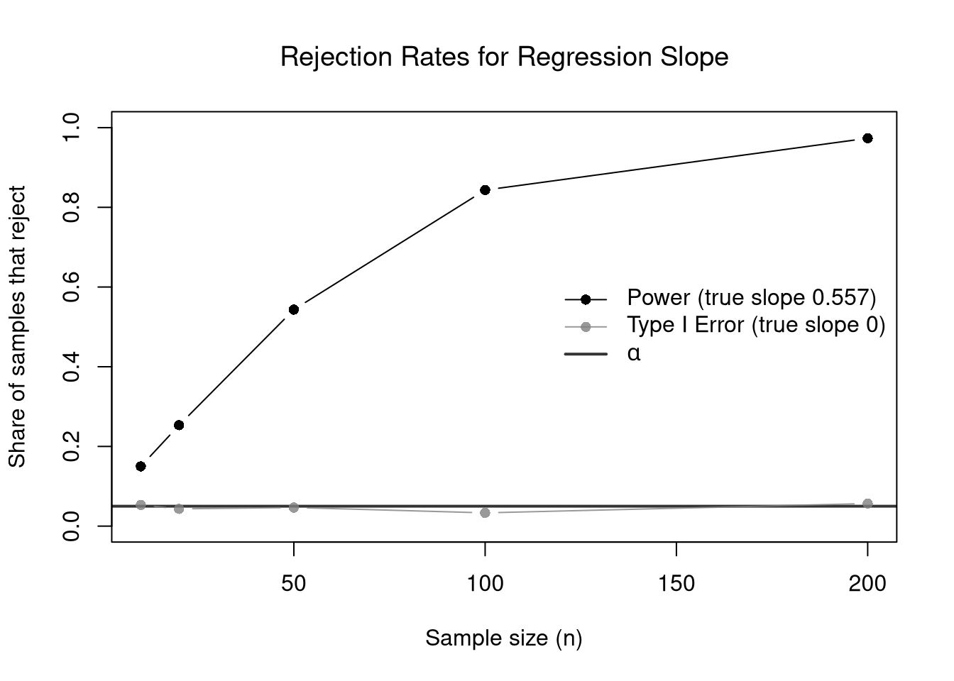
## 0.1500000 0.2533333 0.5433333 0.8433333 0.9733333

# Power with samples of 50 workers
power_est <- power_by_n['50']
To study Type I errors, we need a population where the null is true. Shuffling the outcome once breaks the link between the two variables. By chance, the shuffled population still has a small slope, so we subtract it to make the population slope exactly \(0\). When the true slope is \(0\) (null is true), rejecting is a Type I Error. The share of samples that reject should be near \(\alpha=0.05\) for every sample size.
Code
## MAIN EXAMPLE
# A population where schooling and wages are unrelated
population_null <- population_xy
population_null[, 'y'] <- sample(population_xy[, 'y'])

# Remove the small slope left over by chance
slope_left <- coef(lm(y ~ x, data=population_null))[2]
x_centered <- population_null[, 'x'] - mean(population_null[, 'x'])
population_null[, 'y'] <- population_null[, 'y'] - slope_left * x_centered
coef(lm(y ~ x, data=population_null))[2] # zero, up to rounding
##            x
## 1.209224e-17

# Type I Error rate: share of samples that reject, for each sample size
type1_by_n <- rep(NA, length(n_grid))
for (k in seq_along(n_grid)) {
    p_values_null <- replicate(sim_reps, sample_pval(n_grid[k], population_null))
    type1_by_n[k] <- mean(p_values_null < alpha)
}
names(type1_by_n) <- n_grid
type1_by_n
##         10         20         50        100        200
## 0.05333333 0.04333333 0.04666667 0.03333333 0.05666667
Power rises with the sample size, while the Type I Error rate stays near \(\alpha\).
Code
# Rejection rates by sample size
plot(n_grid, power_by_n, type = 'b', pch = 16,
    xlab = 'Sample size (n)', ylab = 'Share of samples that reject',
    ylim = c(0, 1),
    main = NA)
abline(h = alpha, col = rgb(0, 0, 0, .8), lwd = 2) # drawn first, so the Type I Error series stays visible on top
lines(n_grid, type1_by_n, type = 'b', pch = 16, col = grey(0.5, 0.8))
title('Rejection Rates for Regression Slope', font.main = 1)
legend('right', legend = c('Power (true slope 0.557)', 'Type I Error (true slope 0)', expression(alpha)),
    col = c(1, grey(0.5, 0.8), rgb(0, 0, 0, .8)),
    lty = 1, lwd = c(1, 1, 2), pch = c(16, 16, NA), bty = 'n')
Bayesian Updating
The coin flips example used Bayes’ theorem to update a prior belief about one coin after seeing the other. The same formula turns a test result into an updated belief about whether a hypothesis is true.
Each term in the formula has a name:
- \(\text{Prob}(X_{i}=x)\) is the prior probability for \(X_{i}=x\).
- \(\text{Prob}(Y_{i}=y\mid X_{i}=x)\) is the likelihood of seeing \(Y_{i}=y\) if \(X_{i}=x\) is true.
- \(\text{Prob}(X_{i}=x\mid Y_{i}=y)\) is the posterior, your updated probability after seeing \(Y_{i}=y\).
A useful way to remember the structure is “Posterior \(\propto\) Likelihood \(\times\) Prior”. For two states, the posterior odds equal the prior odds times a likelihood ratio.
Bayesian Screening
A common application of Bayes’ theorem is interpreting a positive result from a diagnostic test.
For a binary screening test where \(X_{i}=1\) means “condition present” and \(Y_{i}=1\) means “test positive”:
Prevalence \(\text{Prob}(X_{i}=1)\) is the base rate of the condition in the population.
Sensitivity \(\text{Prob}(Y_{i}=1\mid X_{i}=1)\) is the probability of a positive result when the condition is present.
False positive rate \(\text{Prob}(Y_{i}=1\mid X_{i}=0)\) is the probability of a positive result when it is absent.
Screening is useful for converting test accuracy and base rates into the quantity an individual actually cares about: the posterior \(\text{Prob}(X_{i}=1\mid Y_{i}=1)\), the probability of having the condition given a positive result. The three inputs play different roles: sensitivity and the false positive rate describe the test, while prevalence describes the population. Suppose a screening test has sensitivity \(0.90\), false positive rate \(0.08\), and prevalence \(0.12\). Applying Bayes’ theorem, \[\begin{aligned}
\text{Prob}(X_{i}=1\mid Y_{i}=1)
&=
\frac{0.90\times0.12}{0.90\times0.12 + 0.08\times0.88}
\approx 0.605.
\end{aligned}\] Even with a good test, the posterior depends strongly on prevalence: rare conditions produce many false alarms even when the test is accurate. The fraud-detection example in Bivariate Distributions showed the same pattern with counts: the same flag meant fraud was unlikely when fraud was rare and likely when it was common.
Code
## MAIN EXAMPLE
# States: X in {0, 1}, signal Y in {0, 1}
# Prior Prob(X_i=1)
p_x1 <- 0.12

# Test characteristics
p_y1_x1 <- 0.90
p_y1_x0 <- 0.08

# Law of total probability for Prob(Y_i=1)
p_y1 <- p_y1_x1 * p_x1 + p_y1_x0 * (1 - p_x1)

# Bayes posterior Prob(X_i=1 | Y_i=1)
p_x1_y1 <- (p_y1_x1 * p_x1) / p_y1
p_x1_y1
## [1] 0.6053812

# Also compute Prob(X_i=1 | Y_i=0)
p_y0_x1 <- 1 - p_y1_x1
p_y0_x0 <- 1 - p_y1_x0
p_y0 <- p_y0_x1 * p_x1 + p_y0_x0 * (1 - p_x1)
p_x1_y0 <- (p_y0_x1 * p_x1) / p_y0
p_x1_y0
## [1] 0.01460565
Notice that a positive test result raises the probability of having the condition from \(12\%\) (prior) to about \(60\%\) (posterior). A negative test result lowers it from \(12\%\) to about \(1.5\%\). If prevalence were higher, say \(50\%\), the posterior after a positive test would be \(\frac{0.90 \times 0.50}{0.90 \times 0.50 + 0.08 \times 0.50} = \frac{0.45}{0.49} \approx 0.92\). The same test is far more informative when prevalence is higher.
Posterior for a Regression Slope
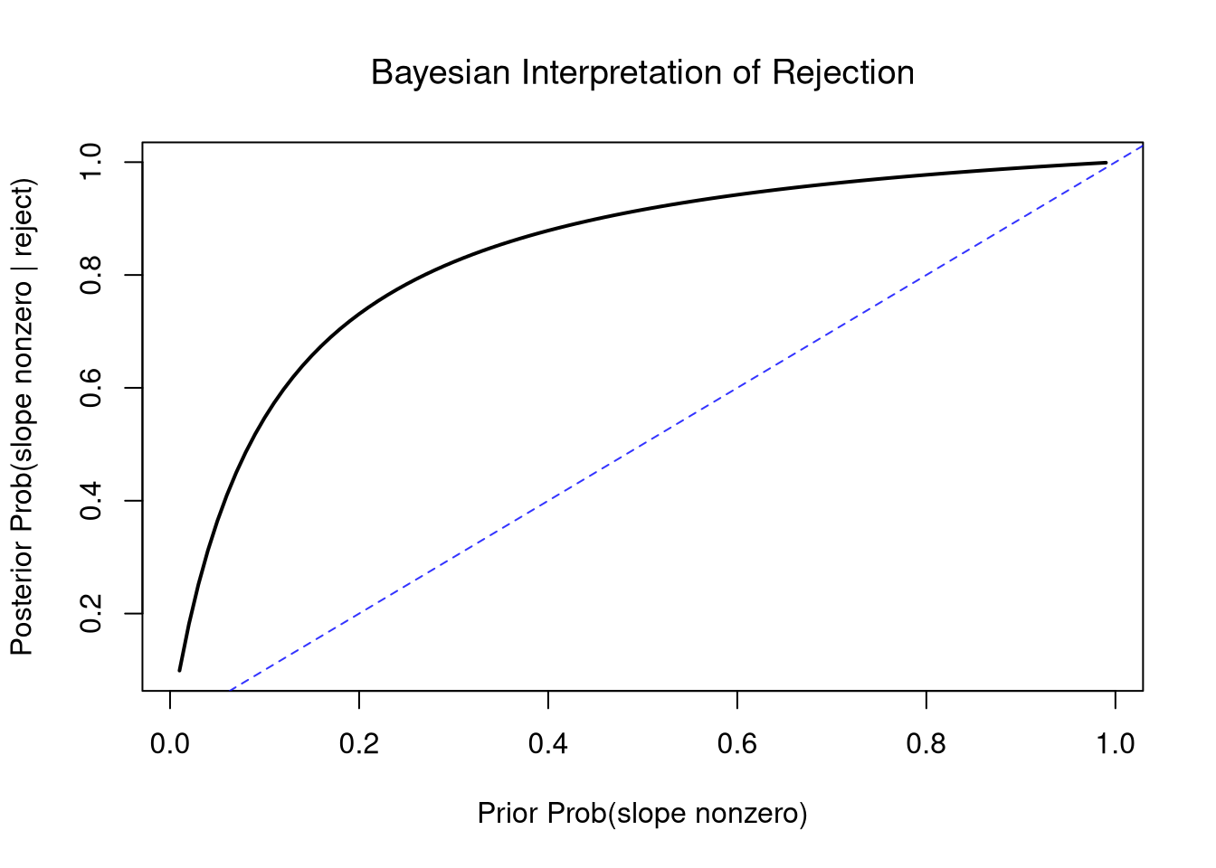
The screening test has the same structure as testing a regression slope. Let \(X_{i}=1\) mean “slope is truly nonzero” and \(Y_{i}=1\) mean “the test rejects \(H_{0}\).” Then sensitivity equals power, the false positive rate equals \(\alpha\), and prevalence is your prior belief that the slope is nonzero. Using the simulation results from the previous section:
Code
# Prior: 50-50 chance the slope is nonzero
prior_nonzero <- 0.5

# 'Sensitivity' = power, 'False positive rate' = alpha
p_reject <- power_est * prior_nonzero + alpha * (1 - prior_nonzero)

# Posterior: Prob(slope nonzero | test rejects)
post_nonzero <- (power_est * prior_nonzero) / p_reject
post_nonzero
##        50
## 0.9157303
Even with moderate power, a rejection substantially updates the posterior probability that the slope is nonzero. A weaker prior (e.g., \(\text{Prob}(\beta_{1} \neq 0) = 0.1\)) would require stronger evidence to reach the same posterior.
Code
# How the posterior changes with different priors
prior_grid <- seq(0.01, 0.99, by = 0.01)
post_grid <- (power_est * prior_grid) /
    (power_est * prior_grid + alpha * (1 - prior_grid))

plot(prior_grid, post_grid, type = 'l', lwd = 2,
    xlab = 'Prior Prob(slope nonzero)',
    ylab = 'Posterior Prob(slope nonzero | reject)',
    main = NA)
title('Bayesian Interpretation of Rejection', font.main = 1)
abline(a = 0, b = 1, col = rgb(0, 0, 1, .8), lty = 2)
Exercises
Comment the script you wrote for this chapter, then restart R and check that it runs from a clean session, then check the script with AI as explained in Working with AI. Write three sentences from memory on the main statistical idea of this chapter, and ask the assistant what is wrong, vague, or missing. Finish with your own questions about whatever you found hardest.
Two joint distributions can have identical marginal distributions but different conditional distributions. Construct a \(2 \times 2\) probability table where \(\text{Prob}(X_{i}=0) = \text{Prob}(X_{i}=1) = 1/2\) and \(\text{Prob}(Y_{i}=0) = \text{Prob}(Y_{i}=1) = 1/2\), but the variables are not independent. Verify by checking whether \(\text{Prob}(X_{i}=x, Y_{i}=y) = \text{Prob}(X_{i}=x)\text{Prob}(Y_{i}=y)\) holds.
Consider a bivariate random vector with the following joint distribution:
Joint Distribution of \(X_{i}\) and \(Y_{i}\)
| \(y=0\) |
\(0.1\) |
\(0.2\) |
\(0.1\) |
| \(y=5\) |
\(0.1\) |
\(0.1\) |
\(0.2\) |
| \(y=10\) |
\(0.0\) |
\(0.1\) |
\(0.1\) |
Compute \(\mathbb{E}[Y_{i}\mid X_{i}=x]\) for each value of \(x\). Then compute \(\mathbb{C}[X_{i}, Y_{i}]\) and the Pearson correlation.
Write R code to simulate \(N = 5000\) draws from a bivariate normal distribution with means \(\mathbb{E}[X_{i}] = 0\), \(\mathbb{E}[Y_{i}] = 5\), variances \(\mathbb{V}[X_{i}] = 4\), \(\mathbb{V}[Y_{i}] = 1\), and correlation \(\rho = 0.6\). Plot the draws as a scatterplot and verify that the sample correlation is close to \(0.6\).
Explain the difference between a Type I Error and a Type II Error in the context of testing \(H_{0}: \beta_{1} = 0\) for a regression slope. Why does increasing the sample size \(n\) improve power without changing the significance level \(\alpha\)?
A screening test has sensitivity \(\text{Prob}(Y_{i}=1\mid X_{i}=1) = 0.95\), false positive rate \(\text{Prob}(Y_{i}=1\mid X_{i}=0) = 0.10\), and prevalence \(\text{Prob}(X_{i}=1) = 0.05\). Use Bayes’ theorem to compute the posterior probability \(\text{Prob}(X_{i}=1\mid Y_{i}=1)\). Explain why the posterior is much lower than the sensitivity.
Recall
This chapter defined joint, marginal, and conditional distributions for a random vector, and the bivariate normal. It also defined the conditional expectation \(\mathbb{E}[Y_{i}\mid X_{i}=x]\), the theoretical covariance \(\mathbb{C}[X_{i}, Y_{i}]\) and correlation, and the regression coefficient \(\beta_{1}\) of a linear data generating process. It then used conditional probabilities for the Type I / Type II error distinction with statistical power, and Bayes’ theorem for converting a test rejection into a posterior. The \(3\times 3\) worked example with \(\text{Prob}(X_{i}=x, Y_{i}=y)\) across \(x~\text{in}~\{0, 1, 2\}\) and \(y~\text{in}~\{0, 10, 20\}\) produced a non-monotonic conditional expectation. It fell from \(\mathbb{E}[Y_{i}\mid X_{i}=0]=15\) to \(\mathbb{E}[Y_{i}\mid X_{i}=1]=10\) and rose to \(\mathbb{E}[Y_{i}\mid X_{i}=2]=50/3\), so there is no true \(\beta_{1}\). But the ratio \(\mathbb{C}[X_{i}, Y_{i}]/\mathbb{V}[X_{i}]=10/7\) still gives an upward best-fitting slope. The example shows the gap between \(\mathbb{E}[Y_{i}\mid X_{i}=x]\) and its best linear approximation. The unfair-coin example showed Bayes’ theorem at work: heads on the second coin raised the probability of heads on the first from \(0.4\) to \(0.6\). Treating the Wages1 workers as a population showed both error rates. Samples from the real population estimated power across sample sizes \(n~\text{in}~\{10, 20, 50, 100, 200\}\). Samples from the shuffled population rejected at a rate near \(\alpha\).
Adamson, Jordan, and Lucas Rentschler. 2025.
“How Policing Incentives Affect Crime, Measurement, and Justice.” Economic Inquiry 63 (2): 545–67.
https://doi.org/10.1111/ecin.13270.
Bayes, Thomas. 1763.
“An Essay Towards Solving a Problem in the Doctrine of Chances.” Philosophical Transactions of the Royal Society of London 53: 370–418.
https://doi.org/10.1098/rstl.1763.0053.
Cohen, Jacob. 1988.
Statistical Power Analysis for the Behavioral Sciences. 2nd ed. Lawrence Erlbaum Associates.
https://doi.org/10.4324/9780203771587.
Hodges, J. L., and E. L. Lehmann. 1956.
“The Efficiency of Some Nonparametric Competitors of the \(t\)-Test.” The Annals of Mathematical Statistics 27 (2): 324–35.
https://doi.org/10.1214/aoms/1177728261.
Ioannidis, John P. A., T. D. Stanley, and Hristos Doucouliagos. 2017.
“The Power of Bias in Economics Research.” The Economic Journal 127 (605): F236–65. https://doi.org/
https://doi.org/10.1111/ecoj.12461.
Neyman, Jerzy, and Egon S. Pearson. 1933.
“On the Problem of the Most Efficient Tests of Statistical Hypotheses.” Philosophical Transactions of the Royal Society of London. Series A 231: 289–337.
https://doi.org/10.1098/rsta.1933.0009.
Pearson, Karl. 1896.
“Mathematical Contributions to the Theory of Evolution. III. Regression, Heredity, and Panmixia.” Philosophical Transactions of the Royal Society of London. Series A 187: 253–318.
https://doi.org/10.1098/rsta.1896.0007.