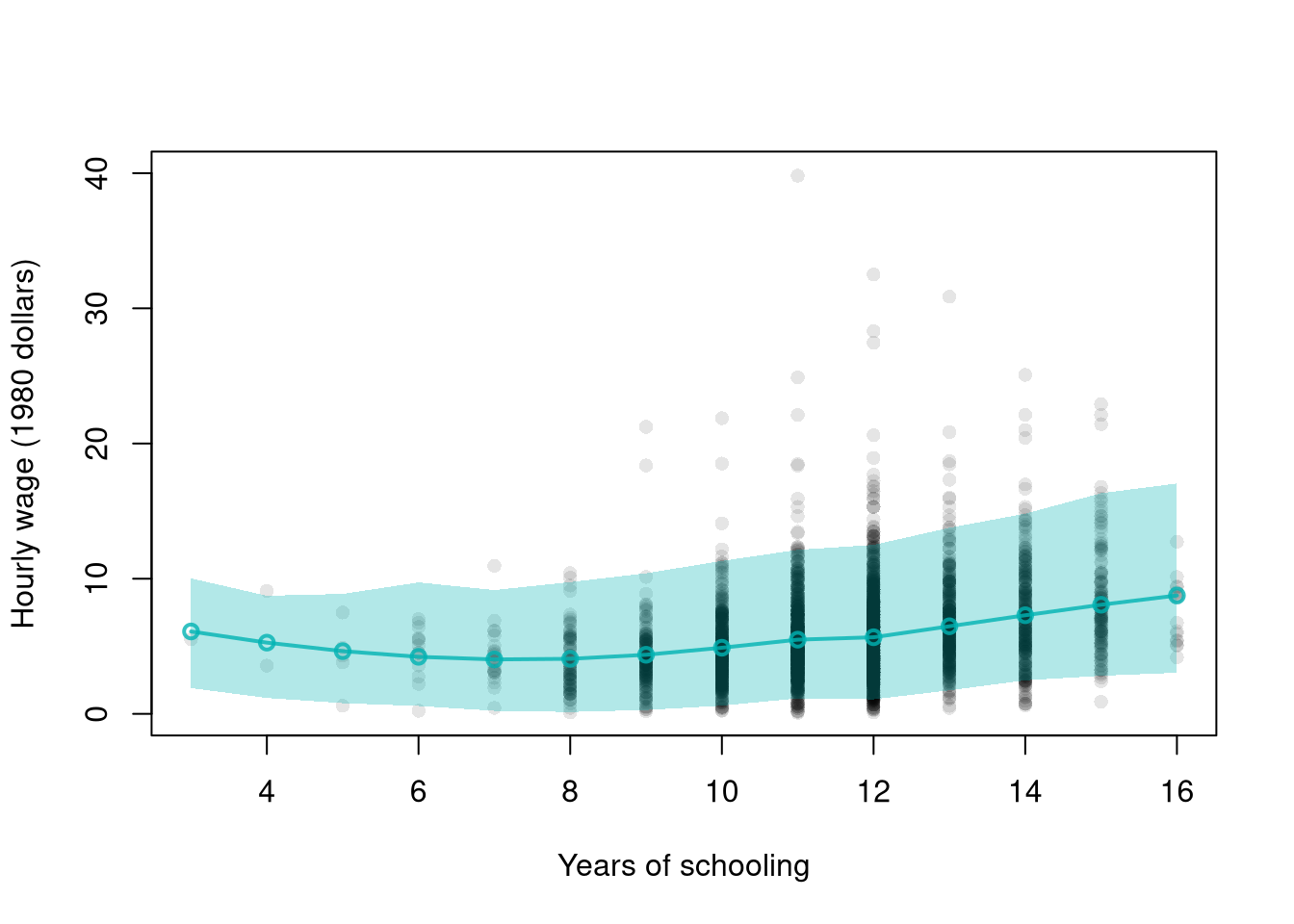
## MAIN EXAMPLE

## Data
# 3294 US workers, with hourly wages in 1980 dollars
data(Wages1, package='Ecdat')
xy_hat <- Wages1[, c('school', 'wage')]
colnames(xy_hat) <- c('x_hat', 'y_hat') # x_hat=years of schooling, y_hat=hourly wage
xy_hat <- xy_hat[order(xy_hat[, 'x_hat']), ]


# Design Points
x_values <- unique(xy_hat[, 'x_hat'])
# Regression
reg_lo <- loess(y_hat ~ x_hat, data=xy_hat, span=.8)
y_pred_lo <- predict(reg_lo, newdata=data.frame(x_hat=x_values))

# Bootstrap Residuals
n <- nrow(xy_hat)
res_lo <- lapply(1:399, function(i){
    xy_boot <- xy_hat[sample(n, replace=TRUE), ]
    reg_b <- loess(y_hat ~ x_hat, data=xy_boot, span=.8)
    resids_b <- resid(reg_b)
    cbind(e_hat=resids_b, x_hat=xy_boot[, 'x_hat'])
})
res_lo <- do.call(rbind, res_lo)

## Smooth residuals
res_fun <- function(x0, h){
    # Include only residuals within h distance to x0
    ki0 <- abs(res_lo[, 'x_hat']-x0)/h
    ki0 <- dunif(ki0)/h
    e_local_hat <- res_lo[ki0 != 0, 'e_hat'] #subset estimates
    ## Local quantiles
    res_i <- quantile(e_local_hat, probs=c(.025, .975), na.rm=TRUE)
    res_i
}
res_ci <- sapply(x_values, res_fun, h=2)

## Prediction Interval
pi_lo1 <- y_pred_lo + res_ci[1, ]
pi_lo2 <- y_pred_lo + res_ci[2, ]

#Plot
plot(y_hat ~ x_hat, pch=16, col=grey(0, .1),
    data=xy_hat, ylim=c(0, 40), main=NA,
    xlab='Years of schooling', ylab='Hourly wage (1980 dollars)')
lines(x_values, y_pred_lo,
    col=rgb(0, .7, .7, .8), lwd=2, type='o')
polygon( c(x_values, rev(x_values)),
    c(pi_lo1, rev(pi_lo2)),
    col=rgb(0, .7, .7, .3), border=NA)