24  Model Assessment

---

A fitted regression should be audited before its coefficients are reported.

This chapter asks two questions.

• Is the fitted model bad in some way?
  • Diagnostic plots: these are four standard model assessment checks from one call to plot().
  • Leverage, standardized residuals, and Cook’s Distance: these find observations that deserve a closer look.
  • Variance Inflation Factor: this measures how much collinearity inflates a coefficient’s variance, \(\hat{\text{VIF}}_{k}=1/(1-\hat{R}^2_{k})\).
  • Normal Q-Q plot and Breusch-Pagan test: these check the residuals, since many tests and default standard errors rely on how the residuals behave.
• Would transforming the data help?
  • Box-Cox transformation: this searches over power transformations that can sometimes rescue a misspecified model.

Before answering either question, look at the raw data with the scatterplot matrices and conditioning plots from Multivariate Distributions. Nonlinear patterns and outliers are often visible before any model is fit. So are explanatory variables that carry almost the same information.

24.1 Model Diagnostics

There’s little sense in getting great standard errors for a terrible model. Plotting your regression object is a simple and easy step to help diagnose whether your model is in some way bad. Calling plot() on an lm object returns four standard plots: (1) residuals vs fitted, (2) Q-Q normal of residuals, (3) scale-location, and (4) residuals vs leverage with Cook’s distance contours. We next go through what each shows.

## MAIN EXAMPLE
# Fit a multiple regression and produce the four standard diagnostic plots.
# Lab data: 3294 US workers.
# wage is the hourly wage in 1980 dollars.
# school and exper are years of schooling and of work experience.
data(Wages1, package='Ecdat')
xy_hat <- Wages1
reg <- lm(wage ~ school + exper, data=xy_hat)
par(mfrow=c(2, 2))
plot(reg, pch=16, col=grey(0, .1))

# The labels beside the most extreme points are row numbers.
# Residuals vs fitted: the smoother stays near 0, but a few residuals are huge.
# Q-Q: the upper tail bends far above the line, since a few wages are very high.
# Scale-location: the smoother rises slowly, so spread grows with the fit.
# Residuals vs leverage: no worker comes near the Cook's contour at 0.5.

Outliers

Some observations sit far from the rest of the data. Eyeballing the plot will not tell us which ones actually move the fit, so we need quantitative tools.

ImportantKey Definition

For a regression with \(n\) observations and \(K\) explanatory variables (so \(K+1\) coefficients):

The leverage \(h_{i}~\text{in}~[0, 1]\) of observation \(i\) measures how unusual its predictor values \(\hat{x}_{i}\) are relative to the rest of the sample. It is small when \(\hat{x}_{i}\) sits near the centre of the predictor cloud and large when \(\hat{x}_{i}\) sits at the edges. Equivalently, \(h_{i}\) is the share of the fitted value \(\hat{y}_{i}^{\mathrm{fit}}\) that is determined by \(\hat{y}_{i}\) itself rather than by the other observations. Across the sample, the \(h_{i}\) sum to the number of coefficients \(K+1\).

The standardized residual \(r_{i} = \hat{e}_{i} / (\hat{s}_{\text{adj}}\sqrt{1-h_{i}})\) rescales the raw residual by an estimate of its standard deviation, where \(\hat{s}_{\text{adj}}\) is the square root of the adjusted mean squared error of the regression.

Cook’s Distance (Cook 1977) sums all prediction changes when observation \(i\) is removed, scaled by the adjusted mean squared error: \[D_{i} = \frac{\sum_{j} \left( \hat{y}^{\mathrm{pred}}(\hat{x}_{j}) - \hat{y}^{\mathrm{pred}(-i)}(\hat{x}_{j}) \right)^2 }{ (K+1) \hat{s}^2_{\text{adj}} } = \frac{\hat{e}_{i}^2}{(K+1) \hat{s}^2_{\text{adj}} } \frac{h_{i}}{(1-h_{i})^2}, \quad \hat{s}^2_{\text{adj}} = \frac{\sum_{i} \hat{e}_{i}^2}{n-K-1}.\] The adjusted mean squared error divides by \(n-K-1\) instead of the \(n\) in the mean squared error, an adjustment for degrees of freedom like the one in the adjusted \(\hat{R}^2\). In Cook’s distance, the argument \(\hat{x}_{j}\) identifies the prediction target and the superscript \((-i)\) identifies the observation omitted from the fit.

These three statistics are useful for finding observations that deserve a closer look. Leverage flags points whose \(\hat{x}_{i}\) is unusual, and the standardized residual flags points whose \(\hat{y}_{i}\) is far from its prediction. Cook’s Distance combines both into one number that says how much the overall fit depends on each observation. The first diagnostic plot (residuals vs fitted) shows outliers in the outcome. The fourth (residuals vs leverage with Cook’s contours) shows outliers in \(\hat{x}_{i}\). Both kinds of outliers can be problematic, but they do not have to be.

N <- 40
x_sim <- c(25, runif(N-1, 3, 8))
e <- rnorm(N, 0, 0.4)
y_sim <- 3 + 0.6*sqrt(x_sim) + e
plot(y_sim ~ x_sim, pch=16, col=grey(0, .5), main=NA)
points(x_sim[1], y_sim[1], pch=16, col=rgb(1, 0, 0, .5))

abline(lm(y_sim ~ x_sim), col=rgb(1, 0, 0, .8), lwd=2)
abline(lm(y_sim[-1] ~ x_sim[-1]), col=rgb(1, 0, 0, .8), lwd=2, lty=2)
legend('topleft', legend=c('All observations', 'Without the red point'),
    col=rgb(1, 0, 0, .8), lwd=2, lty=c(1, 2), bty='n')

NoteMust Know

In the plot above, the red point is a high-leverage observation. How does removing it change the regression line? In your own data analysis, what steps would you take before deciding to remove an outlier?

## MAIN EXAMPLE
# Worker with the highest leverage, shown with its row number
xy_hat[which.max(hatvalues(reg)), ]
##      exper  sex school     wage
## 2102    18 male      3 5.516826
# Row 2102 has 3 years of schooling and 18 of experience, a rare mix.
# Worker with the largest standardized residual
xy_hat[which.max(rstandard(reg)), ]
##      exper  sex school     wage
## 1813     5 male     11 39.80892
# Row 1813 earns about 40 dollars, the highest wage in the data.
# The model predicts only about 5 dollars with 11 years of schooling.

## MAIN EXAMPLE
# Worker with the largest Cook's Distance
xy_hat[which.max(cooks.distance(reg)), ]
##      exper  sex school     wage
## 1813     5 male     11 39.80892
# Row 1813 again: a huge residual, though its leverage is about average.
max(cooks.distance(reg))
## [1] 0.040543
# Still only about 0.04, far below the contour at 0.5.
# So this one worker does not move the fit much.

# Influence plot: leverage vs. standardized residual,
# with point area proportional to Cook's Distance
h_i <- hatvalues(reg)
e_std_hat <- rstandard(reg)
d_i <- cooks.distance(reg)

plot(h_i, e_std_hat, pch=16, col=grey(0, .1),
    cex=1 + 4*d_i/max(d_i), main=NA,
    xlab='Leverage', ylab='Standardized residual')
abline(h=0, col=grey(.5), lty=3)

# Label the most influential observations by row number
inf_id <- order(d_i, decreasing=TRUE)[1:3]
text(h_i[inf_id], e_std_hat[inf_id],
    labels=inf_id, pos=3, cex=.7)

# Row 1813 has a huge residual at ordinary leverage.
# Row 1986 has high leverage, with 4 years of schooling and 18 of experience.
# Row 2490 earns about 22 dollars, with about twice the average leverage.
# So a worker can be influential through the residual, the leverage, or both.

TipTest Yourself

Repeat the outlier checks for lm(Murder ~ Assault + UrbanPop) on USArrests.

# One row per state: arrests per 100,000 residents, and percent urban
# The row names identify the 50 states.
xy2_hat <- USArrests
reg2 <- lm(Murder ~ Assault + UrbanPop, data=xy2_hat)

# State with the highest leverage
which.max(hatvalues(reg2))
## North Carolina 
##             33
# North Carolina has the highest assault rate and few urban residents.
# State with the largest standardized residual
which.max(rstandard(reg2))
## Georgia 
##      10
# Georgia sits about 3 standard deviations above its prediction.
# State with the largest Cook's Distance
which.max(cooks.distance(reg2))
## North Carolina 
##             33
# North Carolina again, through its leverage.
# Its standardized residual is only about -1.3.

# Influence plot: leverage vs. standardized residual,
# with point area proportional to Cook's Distance
h2_i <- hatvalues(reg2)
e2_std_hat <- rstandard(reg2)
d2_i <- cooks.distance(reg2)

plot(h2_i, e2_std_hat, pch=16, col=grey(0, .5),
    cex=1 + 4*d2_i/max(d2_i), main=NA,
    xlab='Leverage', ylab='Standardized residual')
abline(h=0, col=grey(.5), lty=3)

# Label the most influential observations
inf2_id <- order(d2_i, decreasing=TRUE)[1:3]
text(h2_i[inf2_id], e2_std_hat[inf2_id],
    labels=rownames(xy2_hat)[inf2_id], pos=3, cex=.7)

See https://www.r-bloggers.com/2016/06/leverage-and-influence-in-a-nutshell/ for a good interactive explanation, and https://online.stat.psu.edu/stat462/node/87/ for detail. See AEJ-leverage and NBER-leverage for examples of leverage in economics.

Collinearity

When two regressors carry nearly the same information, OLS cannot tell their separate effects apart.

ImportantKey Definition

Collinearity is when one explanatory variable can be closely predicted by a linear combination of the others. The Variance Inflation Factor for variable \(k\), \[\hat{\text{VIF}}_{k}=\frac{1}{1-\hat{R}^2_{k}},\] quantifies how much collinearity inflates the variance of \(\hat{b}_{k}\) compared to the no-collinearity case. Here \(\hat{R}^2_{k}\) comes from regressing \(\hat{x}_{k}\) on the other covariates \(\hat{x}_{-k}\), a regression that does not involve the response variable \(\hat{y}\).

The Variance Inflation Factor is useful as a quick diagnostic for overlapping information between regressors: a \(\hat{\text{VIF}}_{k}\) near \(1\) means \(\hat{x}_{k}\) is uncorrelated with the others, and a common rule of thumb flags \(\sqrt{\hat{\text{VIF}}_{k}} > 2\). Collinearity does not bias the coefficients; it only widens their standard errors so that coefficient estimates may change erratically in response to small changes in the model or the data. In the extreme case with more coefficients than observations (\(K+1>n\)), the linear model has infinitely many solutions.

## MAIN EXAMPLE
# Variance Inflation Factor from its definition: VIF_k = 1/(1 - R^2_k),
# where R^2_k comes from regressing covariate k on the other covariates.
R2_school <- summary(lm(school ~ exper, data=xy_hat))$r.squared
R2_exper  <- summary(lm(exper ~ school, data=xy_hat))$r.squared

vif <- c(school=1/(1-R2_school), exper=1/(1-R2_exper))
vif
##   school    exper 
## 1.038926 1.038926
# Both are about 1.04, as schooling and experience correlate at about -0.19.

# A common rule of thumb flags sqrt(VIF) > 2
sqrt(vif) > 2
## school  exper 
##  FALSE  FALSE
# Neither is flagged, so collinearity is mild in this model.

TipTest Yourself

Repeat the Variance Inflation Factors for lm(Murder ~ Assault + UrbanPop) on USArrests.

xy2_hat <- USArrests
R2_assault  <- summary(lm(Assault ~ UrbanPop, data=xy2_hat))$r.squared
R2_urbanpop <- summary(lm(UrbanPop ~ Assault, data=xy2_hat))$r.squared

vif2 <- c(Assault=1/(1-R2_assault), UrbanPop=1/(1-R2_urbanpop))
vif2
##  Assault UrbanPop 
## 1.071828 1.071828
# Both are about 1.07, as assault rates and urban share correlate at about 0.26.

# A common rule of thumb flags sqrt(VIF) > 2
sqrt(vif2) > 2
##  Assault UrbanPop 
##    FALSE    FALSE
# Neither is flagged.

NoteMust Know

A \(\hat{\text{VIF}}_{k}\) of \(1\) means covariate \(k\) is uncorrelated with the others. A \(\hat{\text{VIF}}_{k}\) of \(4\) means the variance of \(\hat{b}_{k}\) is \(4\) times larger than it would be with no collinearity, so its standard error is \(\sqrt{4}=2\) times larger. With only two covariates, \(\hat{R}^2_{1} = \hat{R}^2_{2}\) (it is just their squared correlation), so the two VIFs are equal. Collinearity does not bias the coefficients; it only makes them less precise.

Normality

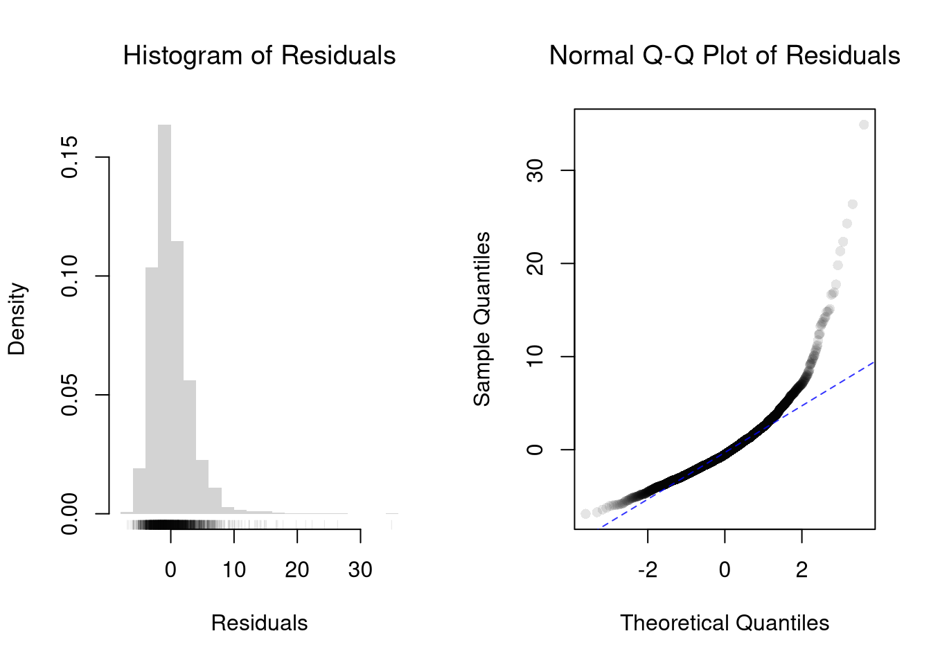
The second diagnostic plot (Q-Q normal of residuals) examines whether the residuals are normally distributed. Your OLS coefficient estimates do not depend on the normality of the residuals. (Good thing, because there’s no reason the residuals of economic phenomena should be so well behaved.) Many hypothesis tests are, however, affected by the distribution of the residuals. For these reasons, you may be interested in assessing normality.

## MAIN EXAMPLE
par(mfrow=c(1, 2))
# The axis keeps every residual, since the long tail is the point here.
hist(resid(reg), breaks=25, border=NA, freq=FALSE,
    main=NA, xlab='Residuals')
rug(resid(reg), col=grey(0, .1))
title('Histogram of Residuals', font.main=1)

qqnorm(resid(reg),
    main='Normal Q-Q Plot of Residuals',
    font.main=1, col=grey(0, .1), pch=16)
qqline(resid(reg), col=rgb(0, 0, 1, .8), lty=2)

# The residuals are right-skewed, with a long tail from a few very high wages.
# The Q-Q points rise far above the line in the upper tail.
# The lower tail is shorter than normal, since wages cannot fall below zero.
# So normality clearly fails here.

#shapiro.test(resid(reg))

TipTest Yourself

Repeat the normality checks for lm(Murder ~ Assault + UrbanPop) on USArrests. How do these residuals compare with the ones above?

xy2_hat <- USArrests
reg2 <- lm(Murder ~ Assault + UrbanPop, data=xy2_hat)

par(mfrow=c(1, 2))
hist(resid(reg2), breaks=15, border=NA, freq=FALSE,
    main=NA, xlab='Residuals')
rug(resid(reg2), col=grey(0, .5))
title('Histogram of Residuals', font.main=1)

qqnorm(resid(reg2),
    main='Normal Q-Q Plot of Residuals',
    font.main=1, col=grey(0, .5), pch=16)
qqline(resid(reg2), col=rgb(0, 0, 1, .8), lty=2)

# The Q-Q points stay close to the line, apart from the largest few residuals.
# The largest, about 7.6, belongs to Georgia.

Heteroskedasticity

OLS treats the error variance as constant across observations, and when that assumption fails the coefficients are still fine but the standard errors are not.

ImportantKey Definition

Heteroskedasticity is when the variance of the residuals depends on the regressors.

Detecting heteroskedasticity is useful because the standard errors that R reports by default rely on a homoskedasticity assumption. If that assumption fails, every \(p\)-value and confidence interval based on those standard errors is wrong too, and typically too narrow. The third diagnostic plot (scale-location) is the visual check; the Breusch-Pagan test (Breusch and Pagan 1979) below is a numerical alternative, whose \(p\)-value comes from a chi-squared distribution.

## MAIN EXAMPLE
# Breusch-Pagan test for heteroskedasticity, by hand.
# Regress the squared residuals on the original regressors:
# a large n*R^2 signals non-constant variance.
e_sq_hat <- resid(reg)^2
aux <- lm(e_sq_hat ~ school + exper, data=xy_hat)
R2_aux <- summary(aux)$r.squared

# Test statistic n*R^2 ~ chi-squared with K degrees of freedom
n <- nrow(xy_hat)
K <- 2
BP <- n*R2_aux
c(statistic=BP, p.value=1-pchisq(BP, df=K))
##    statistic      p.value 
## 12.994415518  0.001507643
# The statistic is about 13 and the p-value about 0.0015, so the test rejects.
# With n this large, even an auxiliary R^2 of about 0.004 is enough to reject.

TipTest Yourself

Repeat the Breusch-Pagan test for lm(Murder ~ Assault + UrbanPop) on USArrests.

xy2_hat <- USArrests
reg2 <- lm(Murder ~ Assault + UrbanPop, data=xy2_hat)

# Breusch-Pagan test for heteroskedasticity, by hand.
e2_sq_hat <- resid(reg2)^2
aux2 <- lm(e2_sq_hat ~ Assault + UrbanPop, data=xy2_hat)
R2_aux2 <- summary(aux2)$r.squared

# Test statistic n*R^2 ~ chi-squared with K degrees of freedom
n2 <- nrow(xy2_hat)
K2 <- 2
BP2 <- n2*R2_aux2
c(statistic=BP2, p.value=1-pchisq(BP2, df=K2))
## statistic   p.value 
## 1.9072736 0.3853371
# The statistic is about 1.9 and the p-value about 0.39, so no rejection.
# With only 50 states, that does not show the variance is constant.

TipTest Yourself

The Breusch-Pagan test asks whether the residual variance depends on the regressors. A small \(p\)-value is evidence of heteroskedasticity: the spread of the residuals changes with the regressors \(\hat{x}_{k}\). Why does heteroskedasticity leave the OLS coefficients unbiased, but make the usual standard errors unreliable?

24.2 Data Transformations

Transforming variables can often improve your model fit while still estimating it via OLS. This is because OLS only requires the model to be “linear in the parameters”. Under the assumption that the model is correctly specified, the following table is how we can interpret the coefficients of the transformed data. (Note for small changes, \(\Delta \log(x) \approx \Delta x / x = \Delta x \% / 100\).)

Interpreting Coefficients in Log Specifications

Specification	Regressand	Regressor	Derivative	Interpretation (If True)
linear–linear	\(y\)	\(x\)	\(\Delta y = \beta_{1}\cdot\Delta x\)	Change \(x\) by one unit \(\rightarrow\) change \(y\) by \(\beta_{1}\) units.
log–linear	\(\log(y)\)	\(x\)	\(\Delta y \% / 100 \approx \beta_{1} \cdot \Delta x\)	Change \(x\) by one unit \(\rightarrow\) change \(y\) by \(100 \cdot \beta_{1}\) percent.
linear–log	\(y\)	\(\log(x)\)	\(\Delta y \approx \frac{\beta_{1}}{100}\cdot \Delta x \%\)	Change \(x\) by one percent \(\rightarrow\) change \(y\) by \(\frac{\beta_{1}}{100}\) units
log–log	\(\log(y)\)	\(\log(x)\)	\(\Delta y \% \approx \beta_{1}\cdot \Delta x \%\)	Change \(x\) by one percent \(\rightarrow\) change \(y\) by \(\beta_{1}\) percent

TipTest Yourself

Suppose you estimate \(\log(y) = 2.1 + 0.08 \cdot x\). The coefficient \(0.08\) means that a one-unit increase in \(x\) is associated with an approximate \(100 \times 0.08 = 8\%\) increase in \(y\). If instead you estimate \(\log(y) = 1.5 + 0.6 \cdot \log(x)\), the coefficient \(0.6\) is an elasticity: a \(1\%\) increase in \(x\) is associated with a \(0.6\%\) increase in \(y\).

Now recall from micro theory that an additively separable and linear production function is referred to as “perfect substitutes”. With a linear model and untransformed data, you have implicitly modelled the different regressors \(X_{ik}\) as perfect substitutes. Further recall that the “perfect substitutes” model is a special case of the constant elasticity of substitution production function.

Box-Cox Transformation

When linear-linear, log-log, and other named specifications are all plausible, we want one estimation procedure that searches across them rather than committing to one ex ante.

ImportantKey Definition

The Box-Cox transformation (Box and Cox 1964) is a family of power transformations of the outcome (indexed by \(\lambda\)) and the regressors (indexed by \(\rho\)), fit to the regression \(Y^{(\lambda)}_{i} = \beta_{0} + \sum_{k=1}^{K} \beta_{k} X^{(\rho)}_{ik} + \epsilon_{i}\) where \[\begin{aligned} Y^{(\lambda)}_{i} &= \begin{cases} \lambda^{-1}\left[ Y_{i}^{\lambda}- 1\right] & \lambda \neq 0 \\ \log(Y_{i}) & \lambda=0 \end{cases}\\ X^{(\rho)}_{i} &= \begin{cases} \rho^{-1}\left[ X_{i}^{\rho}- 1\right] & \rho \neq 0 \\ \log(X_{i}) & \rho=0 \end{cases}. \end{aligned}\]

The Box-Cox family is useful when no single named specification is obviously right. It nests the above specifications as special cases.

• linear-linear (\(\rho=\lambda=1\))
• linear-log \((\lambda=1, \rho=0)\).
• log-linear \((\lambda=0, \rho=1)\).
• log-log (\(\rho=\lambda=0\))

We let the data choose between linear, log, and intermediate fits by minimizing prediction error on the original scale (Box and Cox 1964; Wooldridge 1992; Adamson 2025). When \(\rho=\lambda\) we get the CES production function, which spans the “perfect substitutes” linear-linear model and the “cobb-douglas” log-log model among others. In this CES case, \(\rho~\text{in}~(-\infty,1]\) controls the substitutability of explanatory variables (\(\rho<0\) is “complementary”). The returns to scale depend on the coefficients as well as on \(\rho\) and \(\lambda\), so \(\lambda\) alone does not set them. In the log-log case, the returns to scale equal \(\sum_{k} \beta_{k}\), and \(\sum_{k} \beta_{k}<1\) is “decreasing returns”.¹

We compute the mean squared error in the original scale by inverting the predictions; \[ \hat{y}_{i}^{\mathrm{fit}} = \begin{cases} \left[ \lambda \cdot \hat{y}_{i}^{\mathrm{fit},(\lambda)} + 1 \right]^{1/\lambda} & \lambda \neq 0 \\ \exp\left( \hat{y}_{i}^{\mathrm{fit},(\lambda)} \right) & \lambda=0 \end{cases}. \]

It is easiest to optimize parameters in a 2-step procedure called concentrated optimization. We first solve for \(\hat{\mathbf{b}}(\rho,\lambda)\) and compute the mean squared error \(\text{MSE}(\rho,\lambda)\). We then find the \((\rho,\lambda)\) which minimizes \(\text{MSE}\).

## MAIN EXAMPLE
# Box-Cox Transformation Function
bxcx <- function( xy, rho){
    if (rho == 0L) {
      log(xy)
    } else if(rho == 1L){
      xy
    } else {
      (xy^rho - 1)/rho
    }
}
bxcx_inv <- function( xy, rho){
    if (rho == 0L) {
      exp(xy)
    } else if(rho == 1L){
      xy
    } else {
     (xy * rho + 1)^(1/rho)
    }
}

# Which Variables
reg <- lm(wage ~ school + exper, data=xy_hat)
X <- xy_hat[, c('school', 'exper')]
y_hat <- xy_hat[, 'wage']

# Simple Grid Search over potential (Rho, Lambda)
rl_df <- expand.grid(rho=seq(-2, 2, by=.5), lambda=seq(-2, 2, by=.5))

# Compute Mean Squared Error
# from OLS on Transformed Data
errors <- apply(rl_df, 1, function(rl){
    Xr <- bxcx(X, rl[[1]])
    y_trans_hat <- bxcx(y_hat, rl[[2]])
    xy_trans_hat <- cbind(wage=y_trans_hat, Xr)
    Regr <- lm(wage ~ school + exper, data=xy_trans_hat)
    y_fit <- bxcx_inv(predict(Regr), rl[[2]])
    e_hat  <- (y_hat - y_fit)
    return(e_hat)
})
rl_df$mse <- colMeans(errors^2)

# Want Small MSE and Interpretable
layout(matrix(1:2, ncol=2), width=c(3, 1), height=c(1, 1))
par(mar=c(4, 4, 2, 0))
plot(lambda ~ rho, rl_df, cex=8, pch=15,
    xlab=expression(rho),
    ylab=expression(lambda),
    col=hcl.colors(25)[cut(1/rl_df$mse, 25)])
# Which min
rl0 <- rl_df[which.min(rl_df$mse), c('rho', 'lambda')]
points(rl0$rho, rl0$lambda, pch=0, col=rgb(0, 0, 0, .8), cex=8, lwd=2)
# Legend
plot(c(0, 2), c(0, 1), type='n', axes=FALSE,
    xlab='', ylab='', cex.main=.8,
    main=expression(frac(1, 'Mean Square Error')))
rasterImage(as.raster(matrix(hcl.colors(25), ncol=1)), 0, 0, 1, 1)
text(x=1.5, y=seq(1, 0, l=10), cex=.5,
    labels=levels(cut(1/rl_df$mse, 10)))

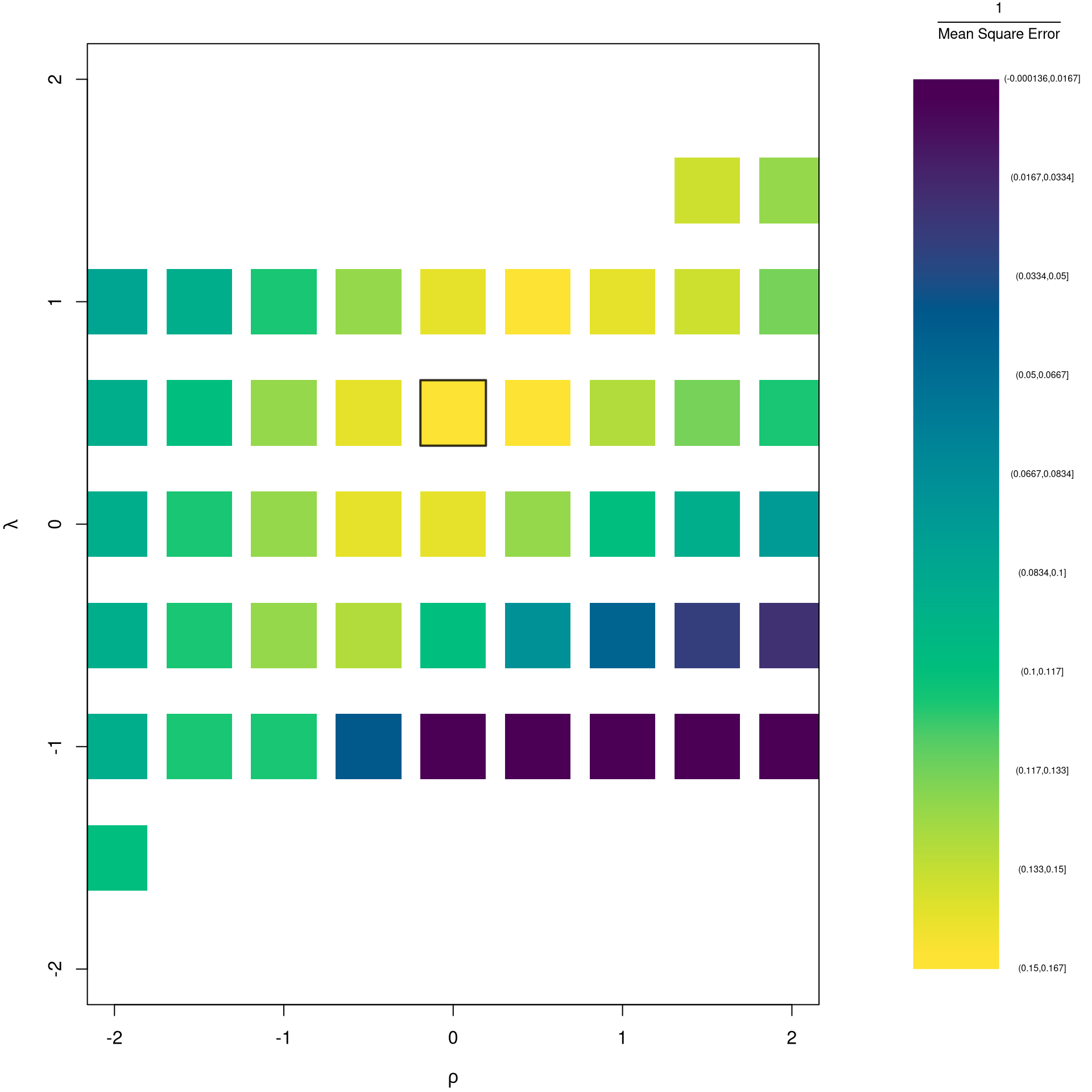
# The box marks the minimum, at rho=2 and lambda=1.
# So wages stay in dollars, and schooling and experience enter squared.
# This is the edge of the grid, but a wider grid finds nothing lower.
# The yellow cells near the box fit about equally well.
# Blank cells have no MSE, since some of their fits cannot be inverted.

NoteMust Know

The grid search finds the \((\rho, \lambda)\) that minimizes MSE. But simple values like \(-1, 0, 1, 2\) are easier to interpret. When might you choose an interpretable transformation over the MSE-minimizing one? What is the trade-off?

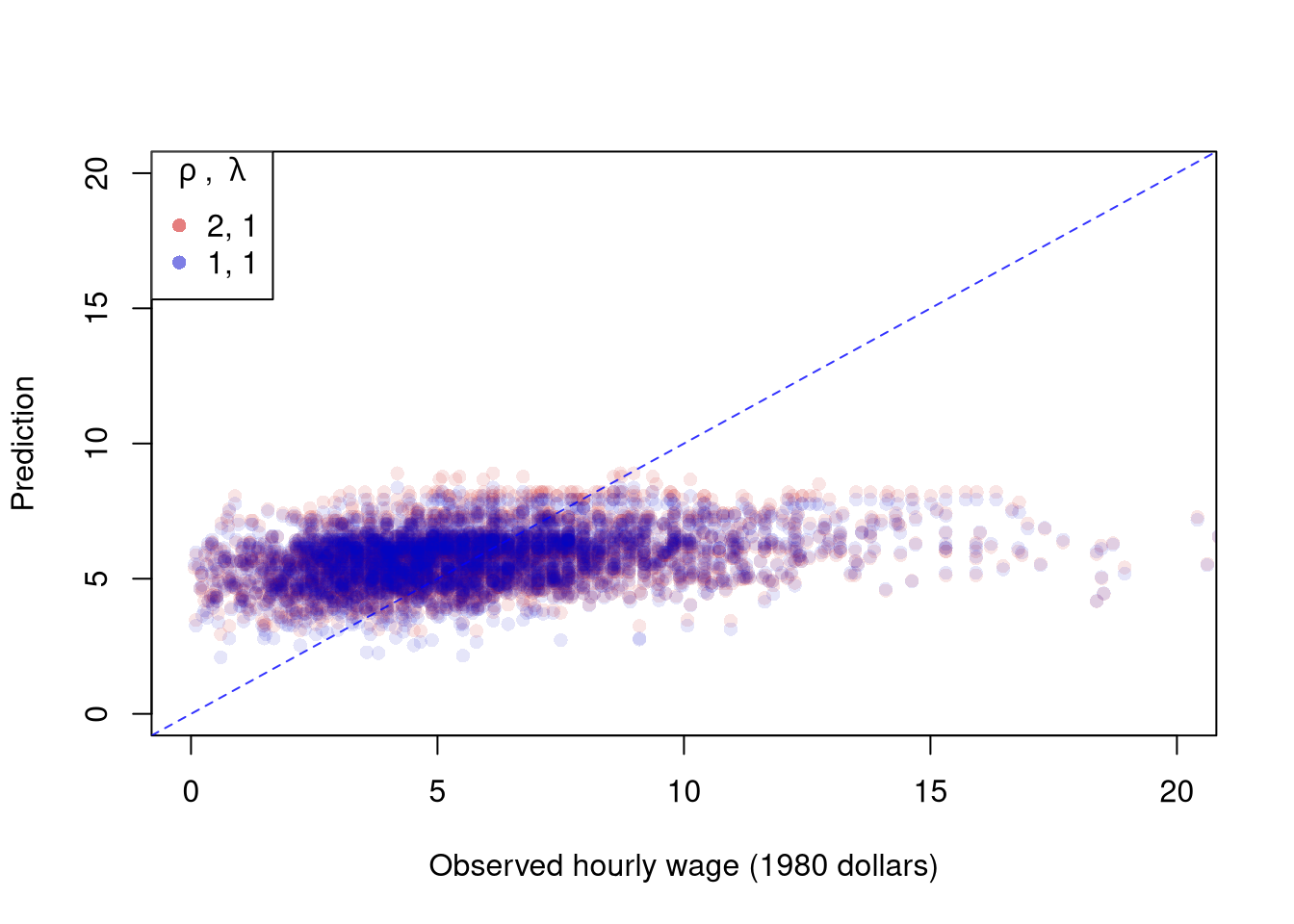
The parameters \(-1,0,1,2\) are easy to interpret and might be selected instead if there is only a small loss in fit. You can also plot the specific predictions to better understand the effect of data transformation beyond mean squared error.

# Plot for Specific Comparisons
Xr <- bxcx(X, rl0[[1]])
y_trans_hat <- bxcx(y_hat, rl0[[2]])
xy_trans_hat <- cbind(wage=y_trans_hat, Xr)
Regr <- lm(wage ~ school + exper, data=xy_trans_hat)
y_fit <- bxcx_inv(predict(Regr), rl0[[2]])

# Faint points, since each model has 3294 of them
pt_cols <- c(rgb(.8, 0, 0, .1), rgb(0, 0, .8, .1))
cols <- c(rgb(.8, 0, 0, .5), rgb(0, 0, .8, .5)) # stronger, for the legend
# The axes stop just past 20 dollars, so the 16 largest wages are not drawn
plot(y_hat, y_fit, pch=16, col=pt_cols[1], ylab='Prediction',
    xlab='Observed hourly wage (1980 dollars)',
    main=NA, xlim=c(0, 20), ylim=c(0, 20))
points(y_hat, predict(reg), pch=16, col=pt_cols[2])
legend('topleft', pch=c(16), col=cols,
    title=expression(rho~', '~lambda),
    legend=c( paste0(rl0, collapse=', '), '1, 1') )
abline(a=0, b=1, col=rgb(0, 0, 1, .8), lty=2)

# Both models predict between about 2 and 9 dollars, while wages reach about 40.
# Their predictions differ by only about 0.12 dollars on average.

We can compare the fit on the original scale: the grid-search optimum versus the untransformed linear baseline.

# Compare prediction MSE on the original wage scale
mse_linear <- mean(resid(reg)^2)
mse_boxcox <- min(rl_df$mse, na.rm=TRUE)
mse_loglog <- rl_df$mse[rl_df$rho == 0 & rl_df$lambda == 0]
c(rl0, mse_linear=round(mse_linear, 3), mse_boxcox=round(mse_boxcox, 3),
    mse_loglog=round(mse_loglog, 3))
## $rho
## [1] 2
## 
## $lambda
## [1] 1
## 
## $mse_linear
## [1] 9.707
## 
## $mse_boxcox
## [1] 9.686
## 
## $mse_loglog
## [1] 10.344
# The grid's best fit, 9.686, beats the linear model, 9.707, by only about 0.2%.
# So the linear model is the easier choice, at a small loss in fit.
# The log-log model, 10.344, fits about 6.6% worse than the linear model.
# On this measure the loss in fit is too large to choose it.
# Most of that gap is bias from undoing the log, since exp() predicts too low.

The grid contains the linear baseline, so its best MSE can only match or beat it. That gain comes at the cost of two extra parameters and a less direct interpretation of the coefficients.

TipTest Yourself

Repeat the grid search and the comparisons for lm(Murder ~ Assault + UrbanPop) on USArrests, using bxcx() and bxcx_inv() from above.

# Which Variables
xy2_hat <- USArrests
reg2 <- lm(Murder ~ Assault + UrbanPop, data=xy2_hat)
X2 <- xy2_hat[, c('Assault', 'UrbanPop')]
y2_hat <- xy2_hat[, 'Murder']

# Simple Grid Search over potential (Rho, Lambda)
rl2_df <- expand.grid(rho=seq(-2, 2, by=.5), lambda=seq(-2, 2, by=.5))

# Compute Mean Squared Error
# from OLS on Transformed Data
errors2 <- apply(rl2_df, 1, function(rl){
    Xr <- bxcx(X2, rl[[1]])
    y_trans_hat <- bxcx(y2_hat, rl[[2]])
    xy_trans_hat <- cbind(Murder=y_trans_hat, Xr)
    Regr <- lm(Murder ~ Assault + UrbanPop, data=xy_trans_hat)
    y_fit <- bxcx_inv(predict(Regr), rl[[2]])
    e_hat  <- (y2_hat - y_fit)
    return(e_hat)
})
rl2_df$mse <- colMeans(errors2^2)

# Want Small MSE and Interpretable
layout(matrix(1:2, ncol=2), width=c(3, 1), height=c(1, 1))
par(mar=c(4, 4, 2, 0))
plot(lambda ~ rho, rl2_df, cex=8, pch=15,
    xlab=expression(rho),
    ylab=expression(lambda),
    col=hcl.colors(25)[cut(1/rl2_df$mse, 25)])
# Which min
rl2 <- rl2_df[which.min(rl2_df$mse), c('rho', 'lambda')]
points(rl2$rho, rl2$lambda, pch=0, col=rgb(0, 0, 0, .8), cex=8, lwd=2)
# Legend
plot(c(0, 2), c(0, 1), type='n', axes=FALSE,
    xlab='', ylab='', cex.main=.8,
    main=expression(frac(1, 'Mean Square Error')))
rasterImage(as.raster(matrix(hcl.colors(25), ncol=1)), 0, 0, 1, 1)
text(x=1.5, y=seq(1, 0, l=10), cex=.5,
    labels=levels(cut(1/rl2_df$mse, 10)))

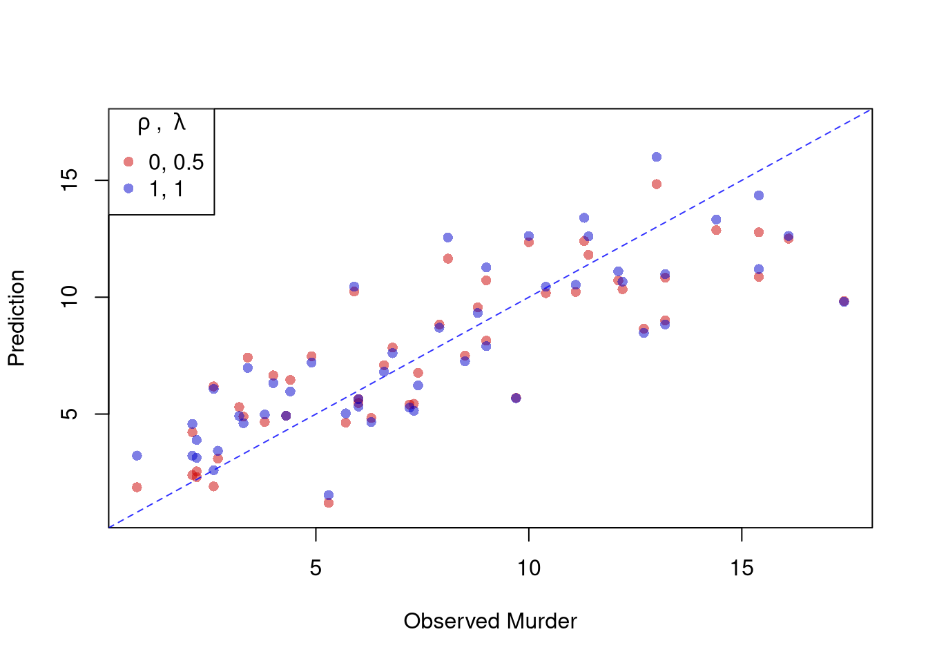
# The box marks the minimum, at rho=0 and lambda=0.5, inside the grid.

# Plot for Specific Comparisons
Xr2 <- bxcx(X2, rl2[[1]])
y2_trans_hat <- bxcx(y2_hat, rl2[[2]])
xy2_trans_hat <- cbind(Murder=y2_trans_hat, Xr2)
Regr2 <- lm(Murder ~ Assault + UrbanPop, data=xy2_trans_hat)
y2_fit <- bxcx_inv(predict(Regr2), rl2[[2]])

cols2 <- c(rgb(.8, 0, 0, .5), rgb(0, 0, .8, .5))
plot(y2_hat, y2_fit, pch=16, col=cols2[1], ylab='Prediction', xlab='Observed Murder',
    main=NA, ylim=range(y2_hat, y2_fit))
points(y2_hat, predict(reg2), pch=16, col=cols2[2])
legend('topleft', pch=c(16), col=cols2,
    title=expression(rho~', '~lambda),
    legend=c( paste0(rl2, collapse=', '), '1, 1') )
abline(a=0, b=1, col=rgb(0, 0, 1, .8), lty=2)

# The two models' predictions differ by about 0.42 arrests on average.

# Compare prediction MSE on the original Murder scale
mse2_linear <- mean(resid(reg2)^2)
mse2_boxcox <- min(rl2_df$mse, na.rm=TRUE)
mse2_loglog <- rl2_df$mse[rl2_df$rho == 0 & rl2_df$lambda == 0]
c(rl2, mse_linear=round(mse2_linear, 3), mse_boxcox=round(mse2_boxcox, 3),
    mse_loglog=round(mse2_loglog, 3))
## $rho
## [1] 0
## 
## $lambda
## [1] 0.5
## 
## $mse_linear
## [1] 6.257
## 
## $mse_boxcox
## [1] 5.999
## 
## $mse_loglog
## [1] 6.446
# The grid's best fit, 5.999, beats the linear model, 6.257, by about 4%.
# The log-log model, 6.446, fits about 3% worse than the linear model.
# So the loss in fit is too large to choose it.

When explicitly transforming data according to \(\lambda\) and \(\rho\), these parameters increase the degrees of freedom by two. The default hypothesis testing procedures do not account for you trying out different transformations, and should be adjusted by the increased degrees of freedom. Specification searches deflate standard errors and are a major source for false discoveries.

Note that if you are ultimately interested in the outcome \(Y_{i}\), then transforming/untransforming \(Y_{i}\) can introduce a bias. To understand when you might be better off sticking with an untransformed outcome variable, see the literature on “smearing”.

24.3 Exercises

1. Comment the script you wrote for this chapter, then restart R and check that it runs from a clean session, then check the script with AI as explained in Working with AI. Write three sentences from memory on the main statistical idea of this chapter, and ask the assistant what is wrong, vague, or missing. Finish with your own questions about whatever you found hardest.

2. A regression has high \(\hat{R}^2\) but one observation has a very large Cook’s Distance. Should you automatically drop that observation? Explain what Cook’s Distance measures and describe a situation where keeping the outlier is the right choice.

3. Using the USArrests dataset, fit lm(Murder ~ Assault + UrbanPop). Produce the four standard diagnostic plots with plot(). Identify the state with the highest leverage (using hatvalues()) and the state with the largest standardized residual (using rstandard()). Are they the same state?

4. Fit the model lm(Murder ~ Assault + UrbanPop, data=USArrests) and then fit a log-linear version lm(log(Murder) ~ Assault + UrbanPop, data=USArrests). Compare the two models by computing the mean squared prediction error in the original (untransformed) scale for each. Which specification fits better?

Further Reading

• https://book.stat420.org/model-diagnostics.html – leverage, Cook’s distance, and residual diagnostics with R examples.
• https://www.econometrics-with-r.org/6-rmwmr.html – interpreting coefficients, specification, and multicollinearity in multiple regression.
• Fox (2020) – a short monograph on influence measures, outliers, and model misspecification.

Recall

This chapter checked a fitted regression with four diagnostic plots for outliers, leverage, normality, and scale. It measured collinearity with the Variance Inflation Factor and tested for heteroskedasticity with the Breusch-Pagan test. It then used Box-Cox transformations to try to rescue a misspecified linear model. The Box-Cox grid-search on wage ~ school + exper made the trade-off concrete: searching over \((\rho, \lambda)\) on \(\{-2, -1.5, \ldots, 2\}^2\) found a fit with MSE \(9.686\) on the original wage scale, barely below the untransformed baseline’s \(9.707\).

Adamson, Jordan. 2025. “Trade and the Rise of Ancient Greek City-States.” Journal of Economic Behavior & Organization 235: 107035. https://doi.org/10.1016/j.jebo.2025.107035.

Bellemare, Marc F., and Casey J. Wichman. 2020. “Elasticities and the Inverse Hyperbolic Sine Transformation.” Oxford Bulletin of Economics and Statistics 82 (1): 50–61. https://doi.org/10.1111/obes.12325.

Box, G. E. P., and D. R. Cox. 1964. “An Analysis of Transformations.” Journal of the Royal Statistical Society: Series B (Methodological) 26 (2): 211–43. https://doi.org/10.1111/j.2517-6161.1964.tb00553.x.

Breusch, T. S., and A. R. Pagan. 1979. “A Simple Test for Heteroscedasticity and Random Coefficient Variation.” Econometrica 47 (5): 1287–94. https://doi.org/10.2307/1911963.

Chen, Jiafeng, and Jonathan Roth. 2024. “Logs with Zeros? Some Problems and Solutions.” The Quarterly Journal of Economics 139 (2): 891–936. https://doi.org/10.1093/qje/qjad054.

Cook, R. Dennis. 1977. “Detection of Influential Observation in Linear Regression.” Technometrics 19 (1): 15–18. https://doi.org/10.1080/00401706.1977.10489493.

Fox, John. 2020. Regression Diagnostics: An Introduction. 2nd ed. Quantitative Applications in the Social Sciences 79. SAGE Publications. https://doi.org/10.4135/9781071878651.

Wooldridge, Jeffrey M. 1992. “Some Alternatives to the Box-Cox Regression Model.” International Economic Review 33 (4): 935–55. https://doi.org/10.2307/2527151.

---

1. One can also use the “shifted” family of Box and Cox. Coefficients from such a regression depend on the units of the outcome, so they should not be read as percentage changes (Bellemare and Wichman 2020; Chen and Roth 2024).