We often want to know the relationship between one outcome variable \(\hat{y}_{i}\) and multiple explanatory variables. This builds on Simple Regression, which related \(\hat{y}_{i}\) to a single \(\hat{x}_{i}\). Multiple linear regression fits a single linear model to several explanatory variables at once, and asks how each one moves the outcome while holding the others fixed.
This chapter asks three questions.
- How is \(\hat{y}\) associated with each explanatory variable, holding the others fixed?
- Multiple regression coefficients: OLS picks one coefficient \(\hat{b}_{k}\) per explanatory variable, with the same objective as simple regression.
- How sure are we?
- Bootstrap standard errors: these assess sampling variability, with the same recipe as the slope.
- Joint bootstrap distribution and permutation \(F\)-test: these assess several coefficients at once. The test shuffles the outcome, the same recipe as earlier permutation tests.
- Adjusted R-squared: this is a new model assessment check that does not reward adding pure noise, unlike R-squared.
- What do the coefficients mean?
- Correctly specified and misspecified simulations: these show that coefficients center on the true values when the data are truly linear. Otherwise, OLS returns the best linear approximation.
For historical reasons, we start by fitting a linear model to data.
The Linear Model
Model and Objective
With several explanatory variables we need a rule for picking one specific coefficient vector out of the infinite candidates that almost fit the data.
The linear model with \(K\) cardinal explanatory variables \(\hat{x}_{i1}, \hat{x}_{i2}, \ldots, \hat{x}_{iK}\) and sample residual \(\hat{e}_{i}\) is \[\begin{aligned}
\hat{y}_{i} &= b_{0} + b_{1} \hat{x}_{i1}+ b_{2} \hat{x}_{i2}+\ldots+b_{K} \hat{x}_{iK} + \hat{e}_{i} = \sum_{k=0}^{K} b_{k} \hat{x}_{ik} + \hat{e}_{i}.
\end{aligned}\] Note that \(\hat{x}_{i0}=1\) in the summation. The coefficients \(b_{k}\) are trial values, and each \(\hat{e}_{i}\) is computed from the observed data for those values.
Ordinary Least Squares (OLS) picks the coefficients that minimize the sum of squared residuals \[\min_{b_{0}, b_{1}, \ldots, b_{K}} \sum_{i=1}^{n} \hat{e}_{i}^2.\]
OLS is useful when you want one coefficient per explanatory variable summarizing its partial relationship with \(\hat{y}\) holding the others fixed; it is the workhorse of linear modeling because the minimization has a closed-form solution via matrix calculations (see these notes for a detailed derivation). The solution yields the best fitting coefficient vector \(\hat{\mathbf{b}}=(\hat{b}_{0} ~~ \hat{b}_{1} ~~... ~~ \hat{b}_{K})\). Plugging it into the model gives the fitted value for observation \(i\): \[\hat{y}_{i}^{\mathrm{fit}} = \sum_{k=0}^{K} \hat{b}_{k} \hat{x}_{ik}.\] At these fitted coefficients, \(\hat{e}_{i} = \hat{y}_{i} - \hat{y}_{i}^{\mathrm{fit}}\) is the observed value minus the fitted value.
Code
## MAIN EXAMPLE
# Lab data: 3294 US workers
# wage is the hourly wage in 1980 dollars
# school and exper are years of schooling and of work experience
# sex is a factor with levels female and male
data(Wages1, package='Ecdat')
xy_hat <- Wages1

# Fit a multiple regression of wage on school and exper
reg <- lm(wage ~ school + exper, data=xy_hat)
coef(reg)
## (Intercept)      school       exper
##  -2.4766831   0.5992289   0.1572607
# With experience fixed, a year of schooling goes with 60 cents more an hour.
# With schooling fixed, a year of experience goes with 16 cents more an hour.

# Compare with schooling alone and with the raw correlations
coef(lm(wage ~ school, data=xy_hat))
## (Intercept)      school
##  -0.7225066   0.5571617
cor(xy_hat[, c('wage', 'school', 'exper')])
##              wage     school       exper
## wage   1.00000000  0.2824925  0.05138051
## school 0.28249249  1.0000000 -0.19356533
## exper  0.05138051 -0.1935653  1.00000000
# Experience barely correlates with wages on its own, about 0.05.
# Its coefficient is still clearly positive once schooling is held fixed.
# Schooling and experience are negatively correlated, about -0.19.
# So holding experience fixed raises the schooling coefficient, 0.557 to 0.599.
Add sex as a third explanatory variable: run lm(wage ~ school + exper + sex, data=xy_hat) and compare the coefficients to those above. R enters this two-level factor as one 0/1 dummy variable, shown as sexmale in the output. Which coefficients change the most? Does the sign of any coefficient change? What does this tell you about the relationship between the explanatory variables?
Goodness of fit
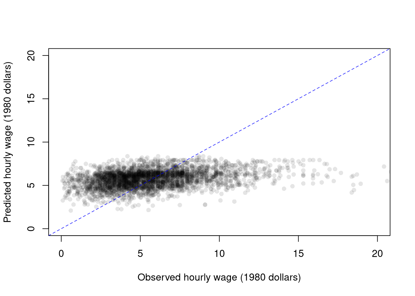
To measure how well the model fits the data, we can again plot our predictions.
Code
# Limits near 20 dollars leave out the 16 largest wages
plot(xy_hat$wage, predict(reg), pch=16, col=grey(0, .1),
    xlim=c(0, 20), ylim=c(0, 20), main=NA,
    xlab='Observed hourly wage (1980 dollars)',
    ylab='Predicted hourly wage (1980 dollars)')
abline(a=0, b=1, col=rgb(0, 0, 1, .8), lty=2)
Code
# Predicted wages span only about 2 to 8 dollars, so the cloud lies flat.
# A close fit would hug the dashed line.
# Here R-squared is about 0.09, so most of the wage variation goes unexplained.
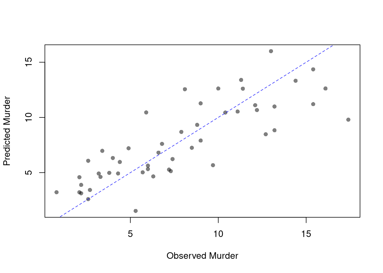
Repeat the plot with USArrests, regressing Murder on Assault and UrbanPop. How close do the points sit to the dashed line, compared to the figure above?
Code
# Second dataset: arrests per 100,000 residents in the 50 US states, 1973
# UrbanPop is the percent of the population living in urban areas
xy2_hat <- USArrests
reg2 <- lm(Murder ~ Assault+UrbanPop, data=xy2_hat)
coef(reg2)
## (Intercept)     Assault    UrbanPop
##  3.20715340  0.04390995 -0.04451047

plot(xy2_hat$Murder, predict(reg2), pch=16, col=grey(0, .5),
    main=NA, xlab='Observed Murder', ylab='Predicted Murder')
abline(a=0, b=1, col=rgb(0, 0, 1, .8), lty=2)
Code
# Predictions track the observed values much more closely.
# R-squared is about 0.66.
Adjusted \(\hat{R}^2\)
The ordinary coefficient of determination is the share of variance the model explains, \(\hat{R}^2 = \frac{\hat{\text{ESS}}}{\hat{\text{TSS}}}=1-\frac{\hat{\text{RSS}}}{\hat{\text{TSS}}}\). Adding extra regressors can mechanically raise the ordinary \(\hat{R}^2\) even when the new variables are pure noise, so we need a fit measure that does not reward including junk.
The adjusted \(\hat{R}^2\) multiplies the unexplained share by a factor that grows with the number of explanatory variables \(K\), \[\hat{R}^2_{\text{adj}} = 1-\frac{n-1}{n-K-1}(1-\hat{R}^2),\] where \(K+1\) counts all estimated coefficients including the intercept (so \(K+1=3\) for a model with two explanatory variables).
The adjusted \(\hat{R}^2\) is useful for comparing models with different numbers of regressors on the same dataset: it rises when an added variable improves fit by more than random noise would. The penalty \((n-1)/(n-K-1)\) is the only thing distinguishing it from the unadjusted version, and it can in fact go negative if the model fits worse than a constant.
Suppose \(n=50\), \(K=2\), and \(\hat{R}^2=0.70\). Then \[\hat{R}^2_{\text{adj}} = 1 - \frac{49}{47}(1-0.70) = 1 - 1.043 \times 0.30 \approx 0.687.\] The adjustment reduces \(\hat{R}^2\) slightly. With more covariates the penalty grows: if instead \(K=9\), then \(\hat{R}^2_{\text{adj}} = 1 - \frac{49}{40}(0.30) = 1 - 0.3675 = 0.6325\).
Code
## MAIN EXAMPLE
# Add pure-noise covariates to a copy, so later chunks still use the original data
ksims <- 1:30
xy_noise_hat <- xy_hat
for(k in ksims){
    xy_noise_hat[, paste0('R', k)] <- runif(nrow(xy_hat), 0, 20)
}
R2_sim <- rep(NA, length(ksims))
R2adj_sim <- rep(NA, length(ksims))
for(k in ksims){
    rvars <- c('school', 'exper', paste0('R', 1:k))
    rvars2 <- paste0(rvars, collapse='+')
    reg_k <- lm( paste0('wage ~ ', rvars2), data=xy_noise_hat)
    R2_sim[k] <- summary(reg_k)$r.squared
    R2adj_sim[k] <- summary(reg_k)$adj.r.squared
}

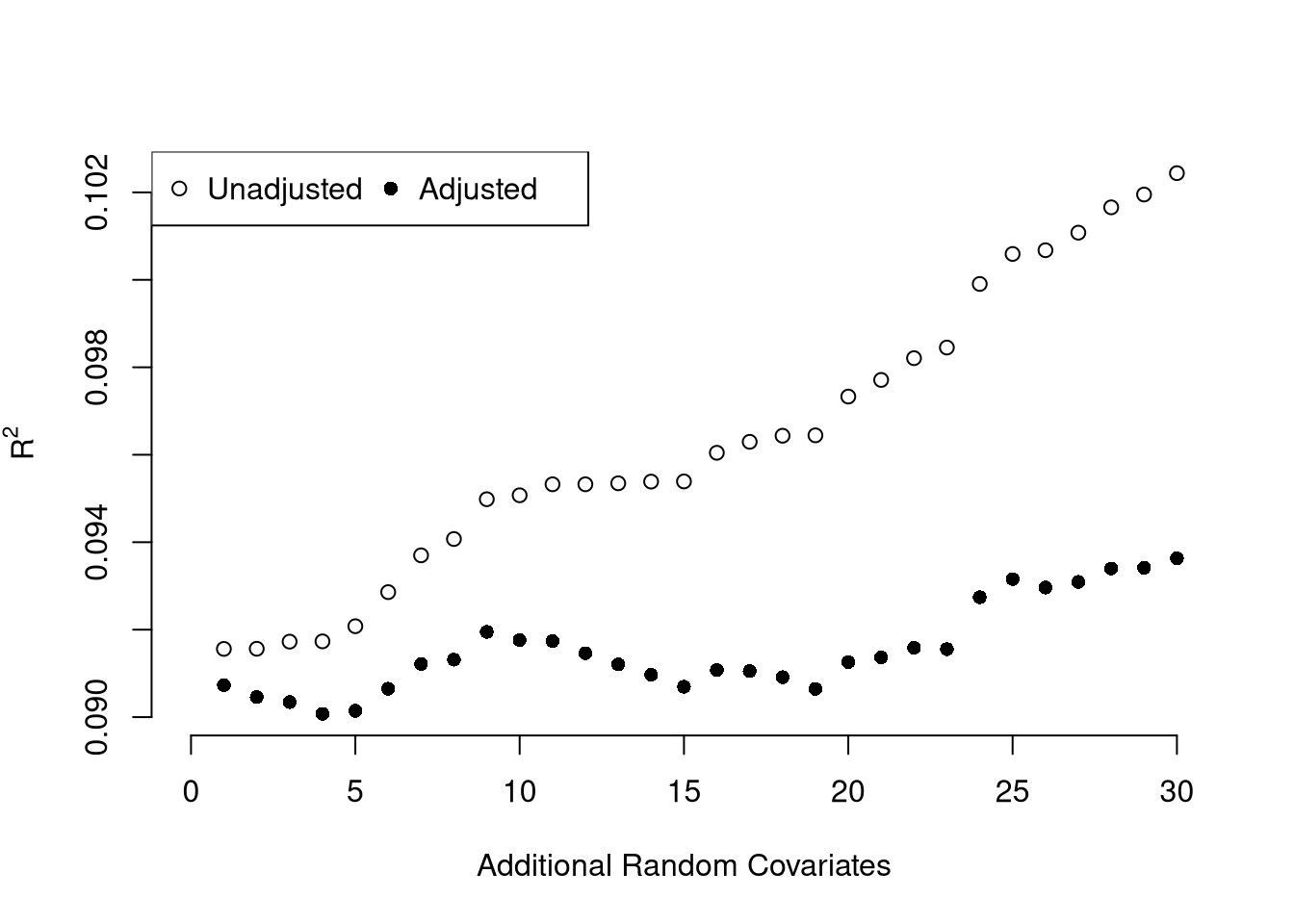
# Zoom in on the y-axis, since noise moves R-squared little with 3294 workers
plot.new()
plot.window(xlim=c(0, 30), ylim=range(R2_sim, R2adj_sim))
points(ksims, R2_sim)
points(ksims, R2adj_sim, pch=16)
axis(1)
axis(2)
mtext(expression(R^2), 2, line=3)
mtext('Additional Random Covariates', 1, line=3)
legend('topleft', horiz=TRUE,
    legend=c('Unadjusted', 'Adjusted'), pch=c(1, 16))
Code
# Pure noise lifts the unadjusted R-squared from about 0.092 to about 0.102.
# The adjusted R-squared stays near 0.09.
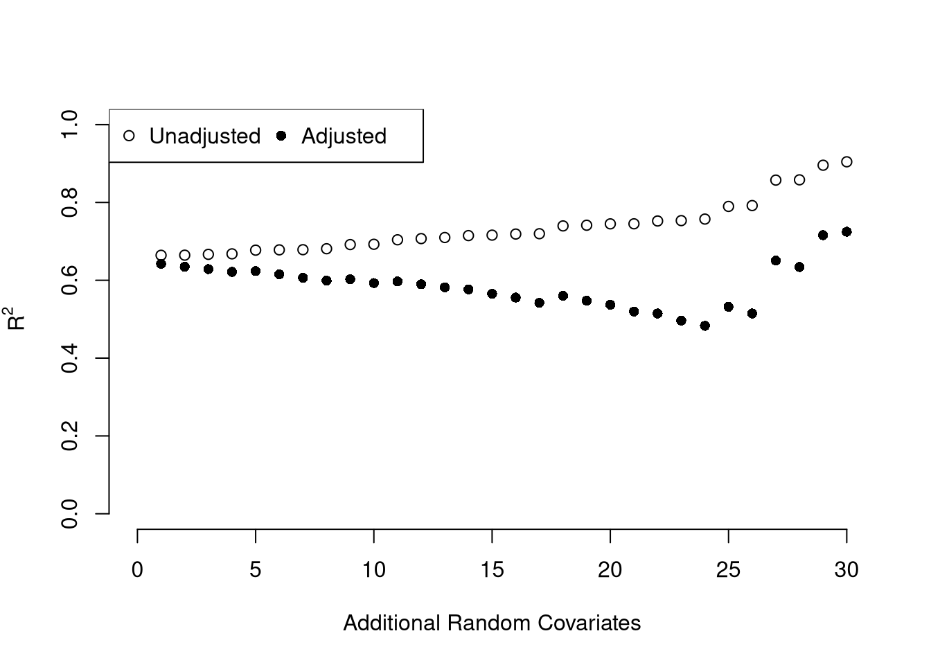
Repeat the simulation with USArrests. How does the number of rows change what noise can do to the unadjusted \(\hat{R}^2\)?
Code
# Second dataset: arrests per 100,000 residents in the 50 US states, 1973
# Its 50 rows are far fewer than the 3294 workers in the lab data.
xy2_hat <- USArrests

# Add pure-noise covariates to a copy, so later chunks still use the original data
ksims <- 1:30
xy2_noise_hat <- xy2_hat
for(k in ksims){
    xy2_noise_hat[, paste0('R', k)] <- runif(nrow(xy2_hat), 0, 20)
}
R2_sim2 <- rep(NA, length(ksims))
R2adj_sim2 <- rep(NA, length(ksims))
for(k in ksims){
    rvars <- c('Assault', 'UrbanPop', paste0('R', 1:k))
    rvars2 <- paste0(rvars, collapse='+')
    reg2_k <- lm( paste0('Murder ~ ', rvars2), data=xy2_noise_hat)
    R2_sim2[k] <- summary(reg2_k)$r.squared
    R2adj_sim2[k] <- summary(reg2_k)$adj.r.squared
}

plot.new()
plot.window(xlim=c(0, 30), ylim=c(0, 1))
points(ksims, R2_sim2)
points(ksims, R2adj_sim2, pch=16)
axis(1)
axis(2)
mtext(expression(R^2), 2, line=3)
mtext('Additional Random Covariates', 1, line=3)
legend('topleft', horiz=TRUE,
    legend=c('Unadjusted', 'Adjusted'), pch=c(1, 16))
Code
# With only 50 states, noise lifts the unadjusted R-squared a lot.
# It climbs from about 0.66 to about 0.9.
# The adjusted R-squared falls to about 0.48 before ending near 0.7.
# With so few rows per covariate, chance fits can move it a lot.
Variability Estimates and Hypothesis Tests
Above, we computed the coefficient vector \(\hat{\mathbf{b}}\) for a particular sample: \(\hat{x}_{i1}, \hat{x}_{i2}, \ldots, \hat{y}_{i}\). We now seek to know how much the estimator \(\mathbf{B}\) varies from sample to sample. I.e., \(\hat{\mathbf{b}}\) is our estimate, and we want the standard errors \(\text{SE}(B_{k})\) of its individual coefficient estimators. We write the estimated standard errors as \(\hat{\text{SE}}(B_{k})\) and compute them using the same data-driven methods introduced previously.
As before, we can also conduct independent hypothesis tests using t-values. However, we can also conduct joint tests that account for interdependencies in our estimates. For example, to test whether two coefficients both equal \(0\), we bootstrap the joint distribution of coefficients.
Code
## MAIN EXAMPLE
# Bootstrap SEs of all three coefficients jointly: resample rows of the
# dataset with replacement, refit lm, and store the coefficient vector.
boot_coefs <- matrix(NA, nrow=399, ncol=3)
for(b in seq(nrow(boot_coefs))){
    b_id <- sample( nrow(xy_hat), replace=TRUE)
    xy_boot <- xy_hat[b_id, ]
    reg_b <- lm(wage ~ school + exper, data=xy_boot)
    boot_coefs[b, ] <- coef(reg_b)
}
colnames(boot_coefs) <- names(coef(reg))

# The bootstrap SE is just the standard deviation across replications
apply(boot_coefs, 2, sd)
## (Intercept)      school       exper
##  0.48176469  0.03443589  0.02451051
# The SEs are about 0.034 for school and 0.025 for exper.
# Both are small next to the coefficients, 0.599 and 0.157.
Joint Hypothesis Tests
When coefficient estimates are correlated, testing them one at a time can miss dependencies that a joint test captures.
A joint hypothesis test asks whether several coefficients are simultaneously consistent with a stated null (e.g., \(\beta_{1} = \beta_{2} = 0\)). The bootstrap above approximates the joint sampling distribution of \(\mathbf{B}\), so we can read off the joint distribution rather than just the marginals.
A joint test is useful when two coefficients move together across resamples: pooling the evidence into one test reflects the actual joint uncertainty, whereas two separate \(t\)-tests would either double-count or miss the dependence entirely. A joint test is also preferable to tests of single coefficients when multicollinearity makes the individual coefficient estimates highly variable (Belsley et al. 1980; Fox 2020). The plot below visualizes the bootstrap joint distribution of two coefficients, where each point is one bootstrap replicate.
Code
## MAIN EXAMPLE
# The joint distribution of the exper and school coefficients
boot_coef_df <- as.data.frame(cbind(
    ID=seq(nrow(boot_coefs)),
    boot_coefs))
fig <- plotly::plot_ly(boot_coef_df,
    type = 'scatter', mode = 'markers',
    x = ~ exper, y = ~ school,
    text = ~ paste('<b> bootstrap dataset: ', ID, '</b>',
            '<br>Coef. exper :', round(exper, 3),
            '<br>Coef. school :', round(school, 3),
            '<br>Coef. Intercept :', round(`(Intercept)`, 3)),
    hoverinfo='text',
    showlegend=FALSE,
    marker=list( color='rgba(0, 0, 0, 0.5)'))
fig <- plotly::layout(fig,
    showlegend=FALSE,
    title='Joint Bootstrap Distribution of Coefficients',
    xaxis = list(title='exper Coefficient'),
    yaxis = list(title='school Coefficient'))
fig
Code
# The cloud tilts up slightly: the two coefficients tend to move together.
# Their correlation across replicates is about 0.2.
Repeat the joint bootstrap with USArrests, regressing Murder on Assault and UrbanPop. Do the two coefficients move together in the same direction as in the figure above?
Code
# Second dataset: arrests per 100,000 residents in the 50 US states, 1973
xy2_hat <- USArrests
reg2 <- lm(Murder ~ Assault+UrbanPop, data=xy2_hat)

# Bootstrap SEs of all three coefficients jointly: resample rows of the
# dataset with replacement, refit lm, and store the coefficient vector.
boot_coefs2 <- matrix(NA, nrow=399, ncol=3)
for(b in seq(nrow(boot_coefs2))){
    b_id <- sample( nrow(xy2_hat), replace=TRUE)
    xy2_boot <- xy2_hat[b_id, ]
    reg2_b <- lm(Murder ~ Assault+UrbanPop, data=xy2_boot)
    boot_coefs2[b, ] <- coef(reg2_b)
}
colnames(boot_coefs2) <- names(coef(reg2))

# The bootstrap SE is just the standard deviation across replications
apply(boot_coefs2, 2, sd)
## (Intercept)     Assault    UrbanPop
##  1.61167232  0.00468114  0.02707630
# The SEs are about 0.005 for Assault and 0.027 for UrbanPop.
# So the UrbanPop coefficient, about -0.045, lies within two SEs of 0.

# The joint distribution of the UrbanPop and Assault coefficients
# Each point is one bootstrap replicate
boot_coef2_df <- as.data.frame(cbind(
    ID=seq(nrow(boot_coefs2)),
    boot_coefs2))
fig2 <- plotly::plot_ly(boot_coef2_df,
    type = 'scatter', mode = 'markers',
    x = ~ UrbanPop, y = ~ Assault,
    text = ~ paste('<b> bootstrap dataset: ', ID, '</b>',
            '<br>Coef. UrbanPop :', round(UrbanPop, 3),
            '<br>Coef. Assault :', round(Assault, 3),
            '<br>Coef. Intercept :', round(`(Intercept)`, 3)),
    hoverinfo='text',
    showlegend=FALSE,
    marker=list( color='rgba(0, 0, 0, 0.5)'))
fig2 <- plotly::layout(fig2,
    showlegend=FALSE,
    title='Joint Bootstrap Distribution of Coefficients',
    xaxis = list(title='UrbanPop Coefficient'),
    yaxis = list(title='Assault Coefficient'))
fig2
Code
# The cloud tilts down: the two coefficients tend to move in opposite ways.
# Their correlation across replicates is about -0.5.
F-statistic
For a single coefficient we have the \(t\)-statistic; with several restrictions at once we need an analog that combines them into one number.
The \(F\)-statistic compares the residual sum of squares of a restricted and an unrestricted model, scaled by their degrees of freedom. With \(q\) restrictions, residual sum of squares \(\hat{\text{RSS}} = \sum_{i} (\hat{y}_{i} - \hat{y}_{i}^{\mathrm{fit}})^2\), and degrees of freedom \(k_{u}\) unrestricted and \(k_{r}\) restricted, \[\hat{F}_{q} = \frac{(\hat{\text{RSS}}_{r}-\hat{\text{RSS}}_{u})/(k_{u}-k_{r})}{\hat{\text{RSS}}_{u}/(n-k_{u})}.\]
The \(F\)-statistic is useful for testing whether several restrictions on a regression hold simultaneously, by comparing two nested models with one number. The most common such test asks whether \(K\) coefficients are all zero. A large \(\hat{F}\) means the unrestricted model fits much better than the restricted one, beyond what would be expected by chance. The restrictions do not have to set coefficients to zero (Wald 1943; Engle 1984).
If you test whether all \(K\) variables are jointly significant, the restricted model is a simple intercept and \(\hat{\text{RSS}}_{r}=\hat{\text{TSS}}\), and \(\hat{F}_{q}\) can be written in terms of \(\hat{R}^2\): \(\hat{F}_{K} = \frac{\hat{R}^2}{1-\hat{R}^2} \frac{n-K-1}{K}\). The first fraction is the relative goodness of fit, and the second fraction is an adjustment for degrees of freedom (similar to how we adjusted the \(\hat{R}^2\) term before). We can also write this test statistic for whether all variables are statistically significant in terms of the adjusted \(\hat{R}^2\): \[
\hat{F}_{K} = \frac{K + (n-K-1)\hat{R}^2_{\text{adj}}}{K(1 - \hat{R}^2_{\text{adj}})}
\] Notice that \(\hat{F}_{K}=1\) when \(\hat{R}^2_{\text{adj}}=0\), meaning the model does not improve fit beyond what random covariates would achieve. The F-statistic exceeds \(1\) when \(\hat{R}^2_{\text{adj}}>0\) and falls below \(1\) when \(\hat{R}^2_{\text{adj}}<0\).
Suppose \(\hat{R}^2_{\text{adj}}=0.50\), \(K=2\), \(n=50\). Then \[\hat{F}_{K} = \frac{K + (n-K-1)\hat{R}^2_{\text{adj}}}{K(1 - \hat{R}^2_{\text{adj}})} = \frac{2 + (50-2-1)(0.50)}{2(1-0.50)} = \frac{2+23.5}{2 \times 0.5} = \frac{25.5}{1} = 25.5.\] This is well above \(1\), indicating that the model explains substantially more variation than random covariates. You can verify: qf(0.95, 2, 47) \(\approx 3.20\), so \(\hat{F}_{K} = 25.5\) is highly significant.
The anova() function compares two nested models with an F-test. Here we test whether exper adds explanatory power beyond school.
Code
reg_r <- lm(wage ~ school, data=xy_hat)         # restricted
reg_u <- lm(wage ~ school + exper, data=xy_hat) # unrestricted
anova(reg_r, reg_u)
## Analysis of Variance Table
##
## Model 1: wage ~ school
## Model 2: wage ~ school + exper
##   Res.Df   RSS Df Sum of Sq      F    Pr(>F)
## 1   3292 32386
## 2   3291 31974  1    411.31 42.335 8.859e-11 ***
## ---
## Signif. codes:  0 '***' 0.001 '**' 0.01 '*' 0.05 '.' 0.1 ' ' 1
# Experience adds explanatory power: F is about 42 and the p-value is near 0.
# RSS falls only about 1 percent, but 3294 workers make that drop decisive.
The F-statistic compares the drop in \(\hat{\text{RSS}}\) to the adjusted mean squared error of the unrestricted model, \(\hat{s}^2_{\text{adj}}=\hat{\text{RSS}}_{u}/(n-k_{u})\). A large F (small p-value) means the extra variable improves the fit by more than random noise would.
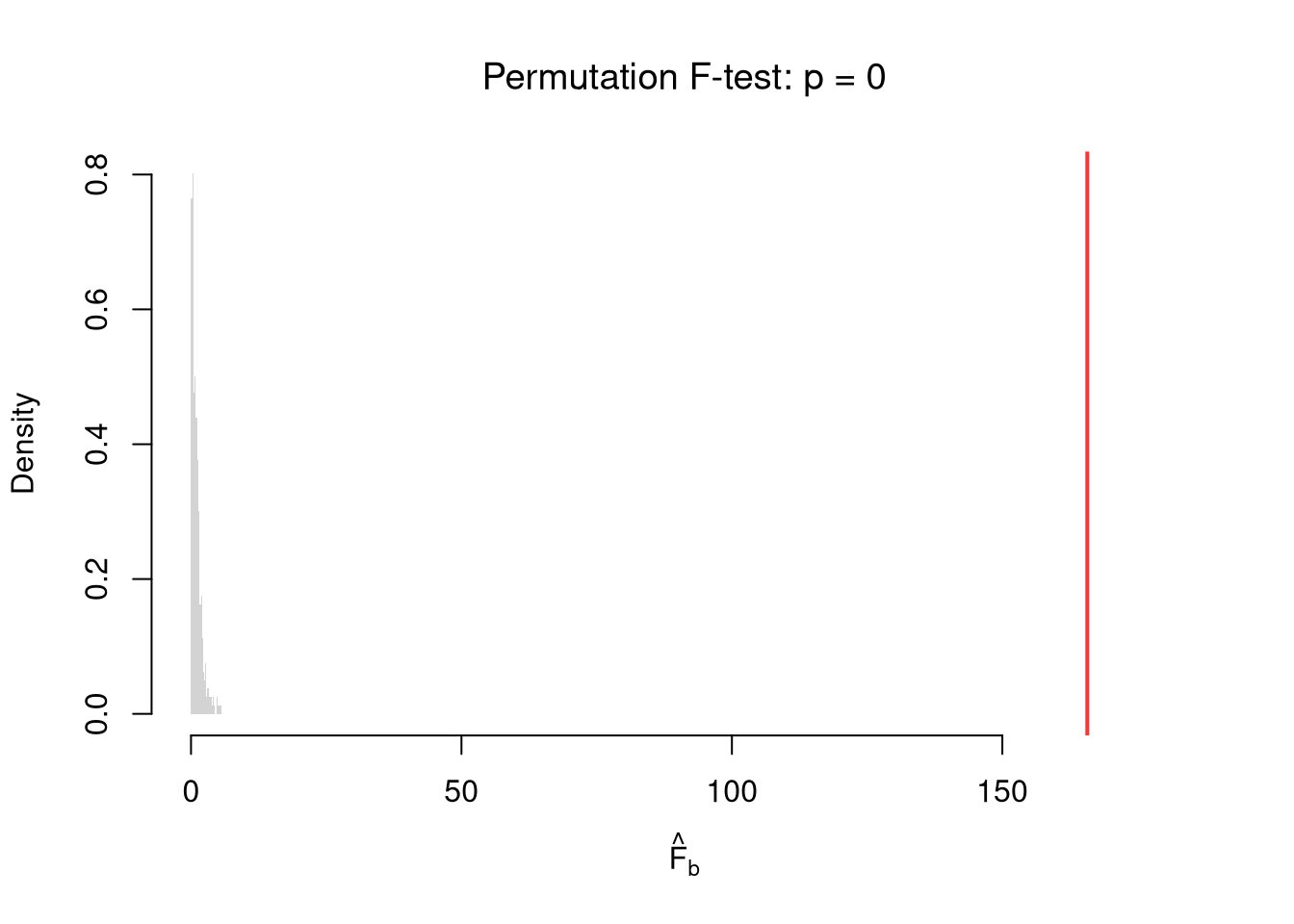
To conduct a hypothesis test, use a permutation test: randomly reshuffle the outcomes, recompute the F statistic each time, and then compare how often shuffled data give something as extreme as your initial statistic. Shuffling the outcome across observations keeps each observation’s covariates together, but breaks the link between the outcome and both covariates, which imposes the null. Here we test whether both slope coefficients are jointly zero in the model above, using the \(\hat{F}_{K}\) that summary() reports.
Code
## MAIN EXAMPLE
# Observed F-statistic, testing whether school and exper are jointly zero
F_hat <- summary(reg)$fstatistic['value']

# Null distribution: shuffle the outcome to break its link with both covariates
F_perm <- rep(NA, 399)
for(b in seq_along(F_perm)){
  # Permuted data
  xy_perm <- xy_hat
  xy_perm$wage <- sample(xy_perm$wage, replace=FALSE)
  # Run regression and store the F-statistic
  reg_b <- lm(wage ~ school + exper, data=xy_perm)
  F_perm[b] <- summary(reg_b)$fstatistic['value']
}
hist(F_perm, xlim=c(0, F_hat*1.1), breaks=25, border=NA,
    freq=FALSE, main=NA, xlab=expression(hat(F)[b]))

# Compare to initial statistic
abline(v=F_hat, lwd=2, col=rgb(1, 0, 0, .8))
p_perm <- mean(F_perm >= F_hat)
title(paste0('Permutation F-test: p = ', round(p_perm, 3)), font.main=1)
Code
# The observed F, about 166, lies far in the right tail.
# The largest of the 399 shuffled F-statistics is only about 5.
Under the null the F-statistic is small, averaging about \(1\) as the formula above predicts when the covariates add nothing.
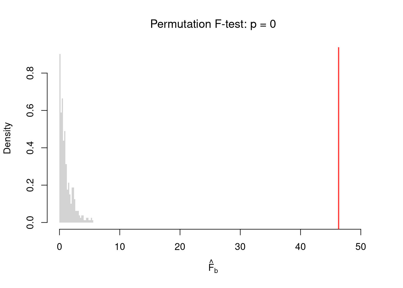
Repeat both tests with USArrests. First use anova() to test whether UrbanPop adds explanatory power beyond Assault. Then run the permutation test of Assault and UrbanPop jointly in Murder ~ Assault + UrbanPop. How can the two tests point in different directions?
Code
# Second dataset: arrests per 100,000 residents in the 50 US states, 1973
xy2_hat <- USArrests
reg2 <- lm(Murder ~ Assault+UrbanPop, data=xy2_hat)

# Test UrbanPop alone, given Assault
reg2_r <- lm(Murder ~ Assault, data=xy2_hat)            # restricted
reg2_u <- lm(Murder ~ Assault + UrbanPop, data=xy2_hat) # unrestricted
anova(reg2_r, reg2_u)
## Analysis of Variance Table
##
## Model 1: Murder ~ Assault
## Model 2: Murder ~ Assault + UrbanPop
##   Res.Df    RSS Df Sum of Sq      F  Pr(>F)
## 1     48 331.85
## 2     47 312.87  1    18.977 2.8507 0.09796 .
## ---
## Signif. codes:  0 '***' 0.001 '**' 0.01 '*' 0.05 '.' 0.1 ' ' 1
# UrbanPop adds little beyond Assault: F is about 2.9 and the p-value about 0.1.

# Observed F-statistic for both coefficients jointly
F2_hat <- summary(reg2)$fstatistic['value']

# Shuffling Murder keeps each state's Assault and UrbanPop together.
# It breaks the link with both covariates, which imposes the null.
F2_perm <- rep(NA, 399)
for(b in seq_along(F2_perm)){
  # Permuted data
  xy2_perm <- xy2_hat
  xy2_perm$Murder <- sample(xy2_perm$Murder, replace=FALSE)
  # Run regression and store the F-statistic
  reg2_b <- lm(Murder ~ Assault+UrbanPop, data=xy2_perm)
  F2_perm[b] <- summary(reg2_b)$fstatistic['value']
}
hist(F2_perm, xlim=c(0, F2_hat*1.1), breaks=25, border=NA,
    freq=FALSE, main=NA, xlab=expression(hat(F)[b]))

# Compare to initial statistic
abline(v=F2_hat, lwd=2, col=rgb(1, 0, 0, .8))
p2_perm <- mean(F2_perm >= F2_hat)
title(paste0('Permutation F-test: p = ', round(p2_perm, 3)), font.main=1)
Code
# The observed joint F, about 46, lies far in the right tail.
# Assault alone already fits well, so the joint test rejects.
# The test of UrbanPop alone asks only about what it adds beyond Assault.
Note that hypothesis testing is not to be done routinely, as additional complications arise when testing multiple hypothesis sequentially.
Under some additional assumptions \(F_{q}\) follows an F-distribution. For more about F-testing, see https://online.stat.psu.edu/stat501/lesson/6/6.2 and https://www.econometrics.blog/post/understanding-the-f-statistic/
Coefficient Interpretation
Notice that we have gotten pretty far without actually trying to meaningfully interpret regression coefficients. That is because the above procedure will always give us a number, regardless of whether the true data generating process is linear or not. So, to be cautious, we have been interpreting the regression outputs while being agnostic as to how the data are generated. We now consider a special situation where we know the data are generated according to a linear process and are only uncertain about the parameter values.
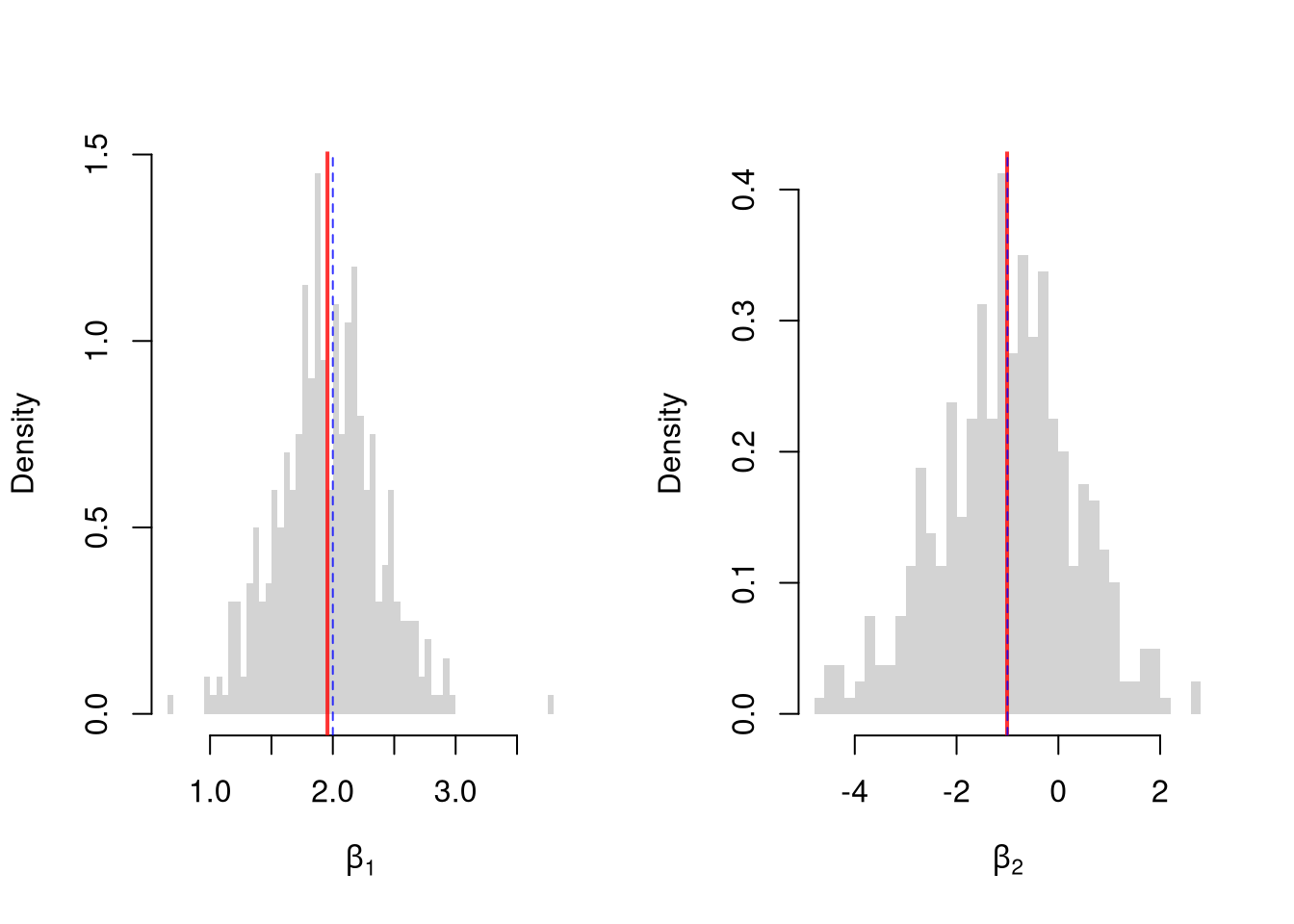
If the data generating process is truly linear then we have a famous result that lets us attach a simple interpretation of OLS coefficients as unbiased estimates of the effect of each \(X_{ik}\). For example, generate a simulated dataset with \(30\) observations and two exogenous variables. Assume the following relationship: \(Y_{i} = \beta_{0} + \beta_{1} X_{i1} + \beta_{2} X_{i2} + \epsilon_{i}\) where the variables and the error term are realizations of the following data generating processes:
Code
N <- 30
beta_true <- c(10, 2, -1)

x1_sim <- runif(N, 0, 5)
x2_sim <- rbinom(N, 1, .7)
X <- cbind(1, x1_sim, x2_sim)
e <- rnorm(N, 0, 3)
y_sim <- X%*%beta_true + e
xy_sim <- data.frame(y_sim, X)
coef(lm(y_sim ~ x1_sim+x2_sim, data=xy_sim))
## (Intercept)      x1_sim      x2_sim
##  10.5710560   1.9817680  -0.9137669
Simulate the distribution of coefficients under a correctly specified model. Interpret the average.
Code
## MAIN EXAMPLE
N <- 30
beta_true <- c(10, 2, -1)

Coefs <- matrix(NA, nrow=3, ncol=400)
for(sim in 1:400){
    x1_sim_b <- runif(N, 0, 5)
    x2_sim_b <- rbinom(N, 1, .7)
    X <- cbind(1, x1_sim_b, x2_sim_b)
    e <- rnorm(N, 0, 3)
    y_sim_b <- X%*%beta_true + e
    xy_sim_b <- data.frame(y_sim_b, x1_sim_b, x2_sim_b)
    Coefs[, sim] <- coef(lm(y_sim_b ~ x1_sim_b+x2_sim_b, data=xy_sim_b))
}

par(mfrow=c(1, 2))
for(i in 2:3){
    hist(Coefs[i, ], breaks=50, xlab=bquote(beta[.(i-1)]), main=NA, border=NA, freq=FALSE)
    abline(v=mean(Coefs[i, ]), lwd=2, col=rgb(1, 0, 0, .8))
    abline(v=beta_true[i], col=rgb(0, 0, 1, .8), lty=2)
}
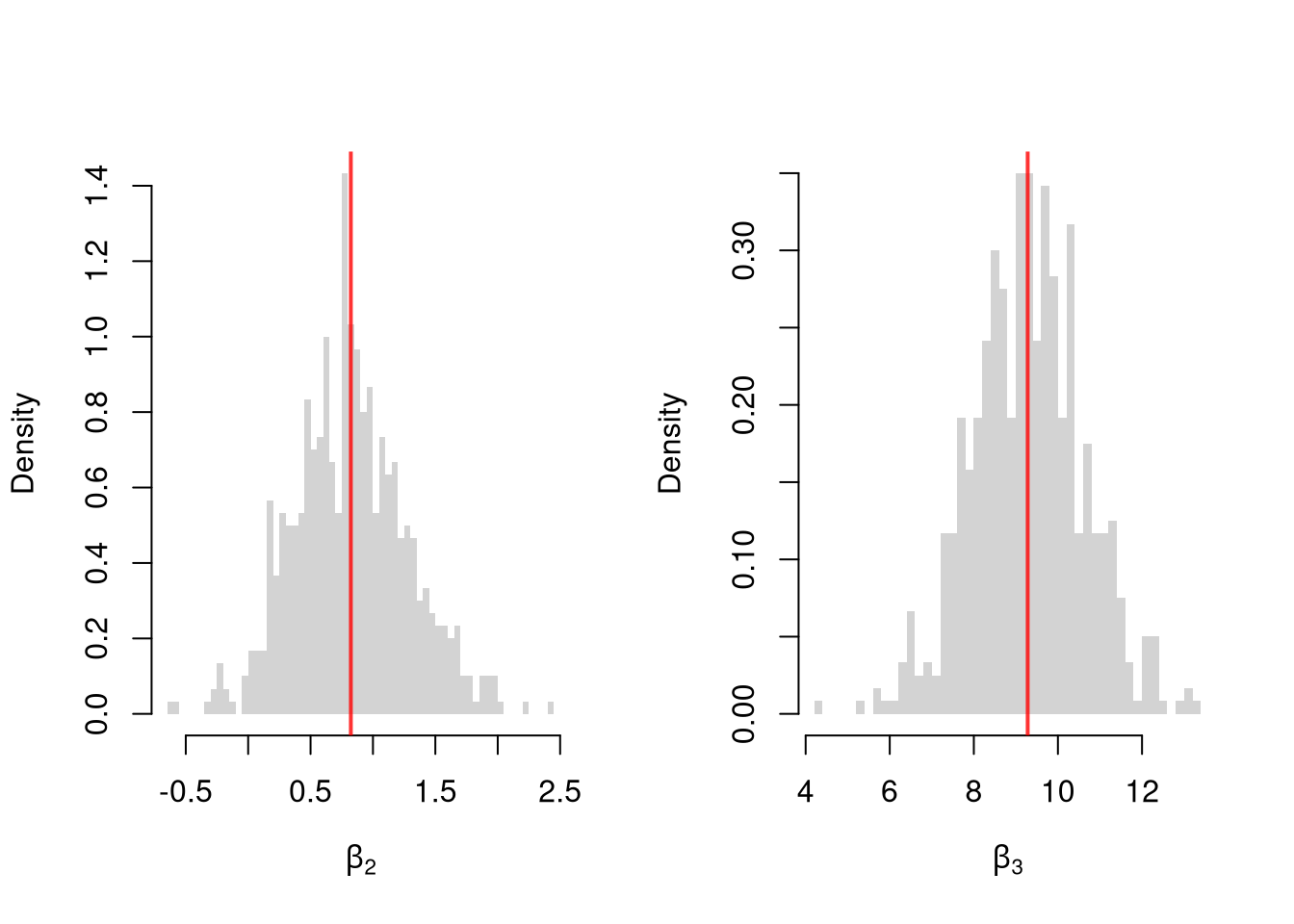
Many economic phenomena are nonlinear, even when including potential transforms of \(\hat{y}\) and \(\hat{x}_{k}\). Sometimes the linear model may still be a good or even great approximation. But sometimes not, and it is hard to know ex-ante. Examine the distribution of coefficients under this misspecified model and try to interpret the average.
Code
## MAIN EXAMPLE
N <- 30

Coefs <- matrix(NA, nrow=3, ncol=600)
for(sim in 1:600){
    x2_sim_b <- runif(N, 0, 5)
    x3_sim_b <- rbinom(N, 1, .7)
    e <- rnorm(N, 0, 3)
    y_sim_b <- 10*x3_sim_b + 2*log(x2_sim_b)^x3_sim_b + e
    xy_sim_b <- data.frame(y_sim_b, x2_sim_b, x3_sim_b)
    Coefs[, sim] <- coef(lm(y_sim_b ~ x2_sim_b+x3_sim_b, data=xy_sim_b))
}

par(mfrow=c(1, 2))
for(i in 2:3){
    hist(Coefs[i, ], breaks=50, xlab=bquote(beta[.(i)]), main=NA, border=NA, freq=FALSE)
    abline(v=mean(Coefs[i, ]), col=rgb(1, 0, 0, .8), lwd=2)
}
In the misspecified case there is no true \(\beta\) for OLS to recover, because the data are not generated by a linear model. The estimated coefficients still have a meaning: OLS returns the linear model that best approximates the true relationship in a least-squares sense. This is why we can still interpret them, cautiously, even when the linear model is wrong.
Compare the two simulation results. In the correctly specified case, the estimated coefficients center on the true values. What happens in the misspecified case? Why might OLS still be useful even when the model is misspecified?
In general, you can interpret your regression coefficients as adjusted correlations: the partial relationship between \(\hat{y}\) and one \(\hat{x}_{k}\) after netting out the linear dependence on the other explanatory variables. There are (many) tests for whether the relationships in your dataset are actually additively separable and linear. A simple way to let a relationship bend is to add the square of an explanatory variable as another regressor (Wooldridge 2019).
\(\hat{R}^2\) vs. \(\hat{b}\)
A small \(\hat{R}^2\) does not mean your coefficients are useless. The two quantities answer different questions: \(\hat{b}_{k}\) tells us how \(\hat{y}\) moves with \(\hat{x}_{k}\), holding other regressors fixed, while \(\hat{R}^2\) tells us how much of the variation in \(\hat{y}\) the model captures. If most of the variation in \(\hat{y}\) comes from things outside the model, \(\hat{R}^2\) will be small even when \(\hat{b}_{k}\) is precisely estimated. For example, wage regressions on years of schooling often report \(\hat{R}^2\) around \(0.1\), yet the schooling coefficient is one of the most studied quantities in labor economics.
That said, we still care about \(\hat{R}^2\). A very small \(\hat{R}^2\) can signal that the model is misspecified (missing important variables or interactions, nonlinear relationships). In this case, you are not actually estimating a theoretical parameter.
Exercises
Comment the script you wrote for this chapter, then restart R and check that it runs from a clean session, then check the script with AI as explained in Working with AI. Write three sentences from memory on the main statistical idea of this chapter, and ask the assistant what is wrong, vague, or missing. Finish with your own questions about whatever you found hardest.
Explain in your own words why \(\hat{R}^2\) can increase when you add a random noise variable to a regression, but \(\hat{R}^2_{\text{adj}}\) generally does not. What does this imply about using \(\hat{R}^2\) alone to choose between models with different numbers of covariates?
Using the USArrests dataset, regress Murder on Assault, UrbanPop, and Rape. Report the \(\hat{R}^2_{\text{adj}}\) and the \(F\)-statistic. Then test whether Rape is jointly significant with the other variables by comparing the full model to a restricted model that excludes Rape.
Using lm(), fit the model Murder ~ Assault + UrbanPop on the USArrests data. Write a bootstrap loop (at least 200 replications) to estimate the standard error of the Assault coefficient. Compare your bootstrap standard error to the one reported by summary().
Recall
This chapter extended simple regression to multiple explanatory variables, with OLS picking one coefficient per variable. With experience fixed, a year of schooling went with about \(60\) cents more an hour. In the \(\hat{R}^2\) vs. adjusted \(\hat{R}^2\) simulation, we added 30 random covariates to wage ~ school + exper. The unadjusted \(\hat{R}^2\) crept upward, while the adjusted version stayed nearly flat. Bootstrap standard errors assessed sampling variability, and a permutation \(F\)-test shuffled the wages to test both slopes jointly. The observed \(\hat{F}\) of about \(166\) lay far above the largest shuffled value of about \(5\). Simulations showed that coefficients center on the true values when the data are truly linear, and that OLS otherwise returns the best linear approximation.
Belsley, David A., Edwin Kuh, and Roy E. Welsch. 1980.
Regression Diagnostics: Identifying Influential Data and Sources of Collinearity. Wiley Series in Probability and Statistics. Wiley.
https://doi.org/10.1002/0471725153.
Engle, Robert F. 1984.
“Wald, Likelihood Ratio, and Lagrange Multiplier Tests in Econometrics.” In
Handbook of Econometrics, vol. 2. Elsevier.
https://doi.org/10.1016/S1573-4412(84)02005-5.
Fox, John. 2020.
Regression Diagnostics: An Introduction. 2nd ed. Quantitative Applications in the Social Sciences 79. SAGE Publications.
https://doi.org/10.4135/9781071878651.
Wald, Abraham. 1943.
“Tests of Statistical Hypotheses Concerning Several Parameters When the Number of Observations Is Large.” Transactions of the American Mathematical Society 54 (3): 426–82.
https://doi.org/10.1090/S0002-9947-1943-0012401-3.