20  Communicating Results

---

Good analysis is only useful to others if its output is clear.

This chapter asks three questions.

• How can readers explore the data for themselves?
  • Interactive figures: these let a reader hover for details, zoom in, and filter the display.
  • Interactive tables: these let a reader search, sort, and filter the rows.
• How do we make a figure easy to read?
  • Data-ink ratio: this is the share of a figure’s ink that displays data, and it guides polishing. We remove details that are not necessary and add details that are.
• How can others rerun our analysis?
  • Quarto reports: these keep prose and code in one file, so rendering regenerates every figure, table, and number.

20.1 Outputs

Interactive Figures

A single static plot fixes one view of the data, but readers often want to explore details the analyst did not pre-select.

ImportantKey Definition

An interactive figure is a plot whose viewer can change the display at runtime (hovering for point-level detail, panning, zooming, or filtering) without re-rendering on the analyst’s side.

Interactive figures are useful when the data have more structure than one static view can show. For example, hovering can reveal labels for many points, and the reader can toggle groups or zoom into a range. The plotly package wraps common plot types (notably histograms, boxplots, and scatterplots) into HTML widgets that work in any browser.

## MAIN EXAMPLE
library('plotly')            # install.packages('plotly')

# Lab data: 3294 US workers.
# wage is the hourly wage in 1980 dollars.
# school and exper are years of schooling and of work experience.
data(Wages1, package='Ecdat')

# Scatter plot of wages vs schooling
fig <- plot_ly(
    Wages1, x = ~ school, y = ~ wage,
    mode='markers',
    type='scatter',
    hoverinfo='text',                              # use custom hover text
    marker=list(color=grey(0, .1)),                # transparent, as n is large
    text = ~ paste('<b>', sex, '</b>',             # one label per worker
        '<br>Schooling :', school,
        '<br>Wage :', round(wage, 2)))
fig <- layout(fig,
    showlegend=FALSE,
    title='Wages and Schooling in America',
    xaxis = list(title = 'Years of schooling'),
    yaxis = list(title = 'Hourly wage (1980 dollars)'))
fig

# Only 52 wages are above 15 dollars.
# To see the rest in more detail, drag a box around them to zoom in.

Color and size can carry two more variables, and the hover text can list every variable for the observation under the cursor. See also https://plotly.com/r/bubble-charts/.

# Bubble chart: color encodes sex and size encodes years of experience
fig <- plot_ly(
    Wages1, x = ~ school, y = ~ wage,
    mode='markers',
    type='scatter',
    hoverinfo='text',
    text = ~ paste('<b>', sex, '</b>',
        '<br>Schooling :', school,
        '<br>Experience :', exper,
        '<br>Wage :', round(wage, 2)),
    color= ~ sex,
    colors=c(rgb(.8, 0, 0), rgb(0, 0, .8)),        # one color per group
    marker=list(
        size= ~ exper,
        opacity=0.1))
fig <- layout(fig,
    title='Wages and Schooling in America',
    xaxis = list(title = 'Years of schooling'),
    yaxis = list(title = 'Hourly wage (1980 dollars)'))
fig

# Click a legend entry to hide or show that group.
# The largest bubbles are at low schooling, where workers have more experience.

TipTest Yourself

Repeat the bubble chart with USArrests, whose rows are named by state. The hover text can then show the name of the state under the cursor.

# 50 US states, 1973: arrests per 100,000 people and percent urban population
xy2_hat <- USArrests
xy2_hat[, 'ID'] <- rownames(xy2_hat) # state name for hover text

# Bubble chart: color and size both encode the murder rate
fig <- plot_ly(
    xy2_hat, x = ~ UrbanPop, y = ~ Assault,
    mode='markers',
    type='scatter',
    hoverinfo='text',
    text = ~ paste('<b>', ID, '</b>',
        '<br>Urban  :', UrbanPop,
        '<br>Assault:', Assault,
        '<br>Murder :', Murder),
    color= ~ Murder,
    marker=list(
        size= ~ Murder,
        opacity=0.5,
        showscale=TRUE,
        colorbar = list(title='Murder Arrests (per 100,000)')))
fig <- layout(fig,
    showlegend=FALSE,
    title='Crime and Urbanization in America 1973',
    xaxis = list(title = 'Percent of People in an Urban Area'),
    yaxis = list(title = 'Assault Arrests per 100,000 People'))
fig

A second trace can add a fitted line, and the hover text can show each observation’s fitted value and residual. The figure below adds the line from a simple regression.

## MAIN EXAMPLE
# Wages and schooling, with the line from a simple regression
xy_hat <- Wages1[, c('school', 'wage')]
colnames(xy_hat) <- c('x_hat', 'y_hat') # x_hat=years of schooling, y_hat=hourly wage
reg <- lm(y_hat ~ x_hat, data=xy_hat)

# Copy the data and attach fitted values and residuals for hover text
xy_plot_hat <- xy_hat
xy_plot_hat[, 'y_fit'] <- predict(reg)
xy_plot_hat[, 'e_hat'] <- resid(reg)

# Plot Data
fig <- plot_ly(
    xy_plot_hat, x = ~ x_hat, y = ~ y_hat,
    mode='markers',
    type='scatter',
    hoverinfo='text',
    marker=list(color=grey(0, .1), size=10),
    text = ~ paste('Schooling :', x_hat,
        '<br>Wage :', round(y_hat, 2),
        '<br>Predicted Wage :', round(y_fit, 2),
        '<br>Residual :', round(e_hat, 2)))
fig <- layout(fig,
    showlegend=FALSE,
    title='Wages and Schooling in America',
    xaxis = list(title = 'Years of schooling'),
    yaxis = list(title = 'Hourly wage (1980 dollars)'))
# Plot Model Predictions as a second trace, with no hover text of its own
fig <- add_trace(fig, x = ~ x_hat, y = ~ y_fit,
    inherit=FALSE, hoverinfo='none',
    mode='lines', type='scatter',
    color=I(rgb(1, 0, 0, .8)),
    line=list(width=2))
fig

# Three schooling groups, as in Comparing Multiple Groups
school_g <- cut(Wages1[, 'school'], breaks=c(0, 11, 12, 16),
    labels=c('<12', '12', '>12'))

# Box Plot
fig <- plot_ly(Wages1,
    y= ~ wage, color= ~ school_g,
    colors=c(rgb(.8, 0, 0), rgb(0, .8, 0), rgb(0, 0, .8)), # one color per group
    alpha=0.6, type='box',
    pointpos=0, boxpoints = 'all',
    marker=list(opacity=0.1),    # transparent points, so the boxes show through
    hoverinfo='text',
    text = ~ paste('<b>', sex, '</b>',
        '<br>Schooling :', school,
        '<br>Experience :', exper,
        '<br>Wage :', round(wage, 2)))
fig <- layout(fig,
    showlegend=FALSE,
    title='Wages and Schooling in America',
    xaxis = list(title = 'Years of schooling',
        type='category'),        # 12 is a group label, not a number
    yaxis = list(title = 'Hourly wage (1980 dollars)', range=c(0, 20)))
fig

# The 18 wages above 20 dollars start off screen.
# Double-click the figure to see them.
# Median wages rise across the groups, at about 4.59, 5.17, and 6.74 dollars.

# Split workers at the mean schooling, about 11.6 years
m_x_hat <- mean(xy_hat[, 'x_hat'])
school_cut <- xy_hat[, 'x_hat'] < m_x_hat
y1_hat <- xy_hat[school_cut, 'y_hat']  # hourly wages, low schooling
y2_hat <- xy_hat[!school_cut, 'y_hat'] # hourly wages, high schooling

# Overlapping Histograms
fig <- plot_ly(alpha=0.6, hovertemplate='%{y}')
fig <- add_histogram(fig, y1_hat, name='Low (< Mean)',
    histnorm = 'probability density',
    xbins = list(start=0, size=1))
fig <- add_histogram(fig, y2_hat, name='High (>= Mean)',
    histnorm = 'probability density',
    xbins = list(start=0, size=1))
fig <- layout(fig,
    barmode='overlay',
    title='Wages and Schooling in America',
    xaxis = list(title='Hourly wage (1980 dollars)', range=c(0, 20)),
    yaxis = list(title='Density'),
    legend=list(title=list(text='<b> Years of Schooling </b>')) )
fig

# The 18 wages above 20 dollars start off screen.
# Both groups are right-skewed.
# The high group sits further right, with a median wage of about 5.73 vs 4.59.

# Possible, but less preferable, to stack histograms
# barmode='stack', histnorm='count'

Note that many plots can be made interactive via https://plotly.com/r/. For more details, see examples and then applications.

If you have many points, for example, you can make a 2D histogram.

fig <- plot_ly(
    xy_hat, x = ~ x_hat, y = ~ y_hat)
fig <- add_histogram2d(fig, nbinsx=25, nbinsy=25)
fig

Interactive Tables

For raw data, a static table forces the analyst to pre-pick which rows the reader sees first.

ImportantKey Definition

An interactive table shows rows of data with built-in filtering, sorting, and search controls. The viewer chooses which rows to see; the analyst does not need to pre-aggregate.

Interactive tables are useful when the reader wants to look up specific records rather than a summary view: searching by row identifier, sorting on a particular column, or filtering down to a subset. The reactable package renders a data frame as an HTML widget with these controls already built in.

## MAIN EXAMPLE
library('reactable')                     # install.packages('reactable')

# Copy the data and round wages to the cent for display
xy_table_hat <- Wages1
xy_table_hat[, 'wage'] <- round(xy_table_hat[, 'wage'], 2)

reactable(xy_table_hat,
    filterable=TRUE,                        # one search box per column
    highlight=TRUE)                         # row highlighting on hover

# The 3294 workers fill many pages, so the table shows ten rows at a time.

You can create an interactive table that summarizes the data too.

# Compute summary statistics for the numeric columns, since sex is a factor
vars <- c('wage', 'school', 'exper')
stats_list <- vector('list', length(vars))
for (i in seq_along(vars)) {
  v <- vars[i]
  x_v_hat <- Wages1[[v]]
  stats_list[[i]] <- c(
    Variable = v,
    N       = sum(!is.na(x_v_hat)),
    Mean    = mean(x_v_hat, na.rm = TRUE),
    SD      = sd(x_v_hat, na.rm = TRUE),
    Min     = min(x_v_hat, na.rm = TRUE),
    Q1      = as.numeric(quantile(x_v_hat, 0.25, na.rm = TRUE)),
    Median  = median(x_v_hat, na.rm = TRUE),
    Q3      = as.numeric(quantile(x_v_hat, 0.75, na.rm = TRUE)),
    Max     = max(x_v_hat, na.rm = TRUE)
  )
}

# Convert list to data frame with numeric columns 
stats_df <- as.data.frame(do.call(rbind, stats_list), stringsAsFactors = FALSE)
num_cols <- setdiff(names(stats_df), 'Variable')
for (col in num_cols) {
    stats_df[[col]] <- round(as.numeric(stats_df[[col]]), 3)
}

# Display interactively
reactable(stats_df)

Polishing

A first-draft figure usually works for the analyst but not for anyone else. Polishing removes what is not data and adds what the reader needs, so the figure is readable at first glance.

ImportantKey Definition

The data-ink ratio is the share of ink in a figure devoted to displaying data: \[\text{data-ink ratio} = \frac{\text{ink used to display data}}{\text{total ink in the figure}}.\] Non-data ink is everything else: gridlines, borders, shading, redundant labels, and decoration.

The data-ink ratio is useful as a one-number guide for polishing. A low ratio means clutter is competing with the data. A high ratio means almost all the ink shows data. Tufte (2001) introduces it to push figures toward a single goal: every mark should help the reader see the data. So erase any element that, if removed, would not change what the reader learns. When polishing, you do two things:

• Add details that are necessary.
• Remove details that are not necessary.

NoteMust Know

Data-Ink Ratio numerical example. Consider a scatter plot of 50 points with a heavy gray background, a thick border, and three duplicate legends. Of all the pixels printed, only the 50 points are data ink. Suppose those points account for 200 pixels and the rest of the figure uses 1800 pixels. The data-ink ratio is \(200/(200 + 1800) = 0.10\). Strip the background, border, and duplicate legends, and the ratio for the same 200 data pixels might be \(200/250 = 0.80\). The figure carries the same information, and its ratio is eight times higher.

The two panels below show the same data. The left panel piles on non-data ink; the right strips it back. The extra ink on the left adds no information about the data.

## MAIN EXAMPLE
par(mfrow=c(1, 2), mar=c(5, 4, 3, 1))

# Cluttered: oversized two-color markers, gridlines, redundant title
plot(y_hat ~ x_hat, data=xy_hat,
    pch=21, bg='red', col='blue', cex=1.5,
    main='Hourly Wage vs Schooling\n(US Workers)',
    sub='Source: Wages1',
    xlab='school (years)',
    ylab='Hourly Wage in 1980 Dollars (wage)')
grid(col='black', lwd=1)
box(lwd=2)
legend('topright', legend='Worker', pch=21, pt.bg='red', col='blue')
# The opaque markers merge into solid columns, hiding where workers pile up.

# Polished: light points, no grid, no redundant labels or legend
plot(y_hat ~ x_hat, data=xy_hat,
    pch=16, col=grey(0, .1),                     # transparent black points
    main=NA, xlab='Years of schooling', ylab='Hourly wage (1980 dollars)',
    bty='n')                                     # drop the surrounding box
title('US Workers', font.main=1, adj=0)

# Schooling is in whole years, so the points form vertical stripes.
# The stripes are darkest where workers pile up, above all at 12 years.
# Wages tend to rise with schooling, though weakly (correlation about 0.28).

Removed: oversized two-color markers, grid, box, redundant title, subtitle, one-entry legend. Added: nothing; the cleaner panel reads faster because nothing competes with the points.

TipTest Yourself

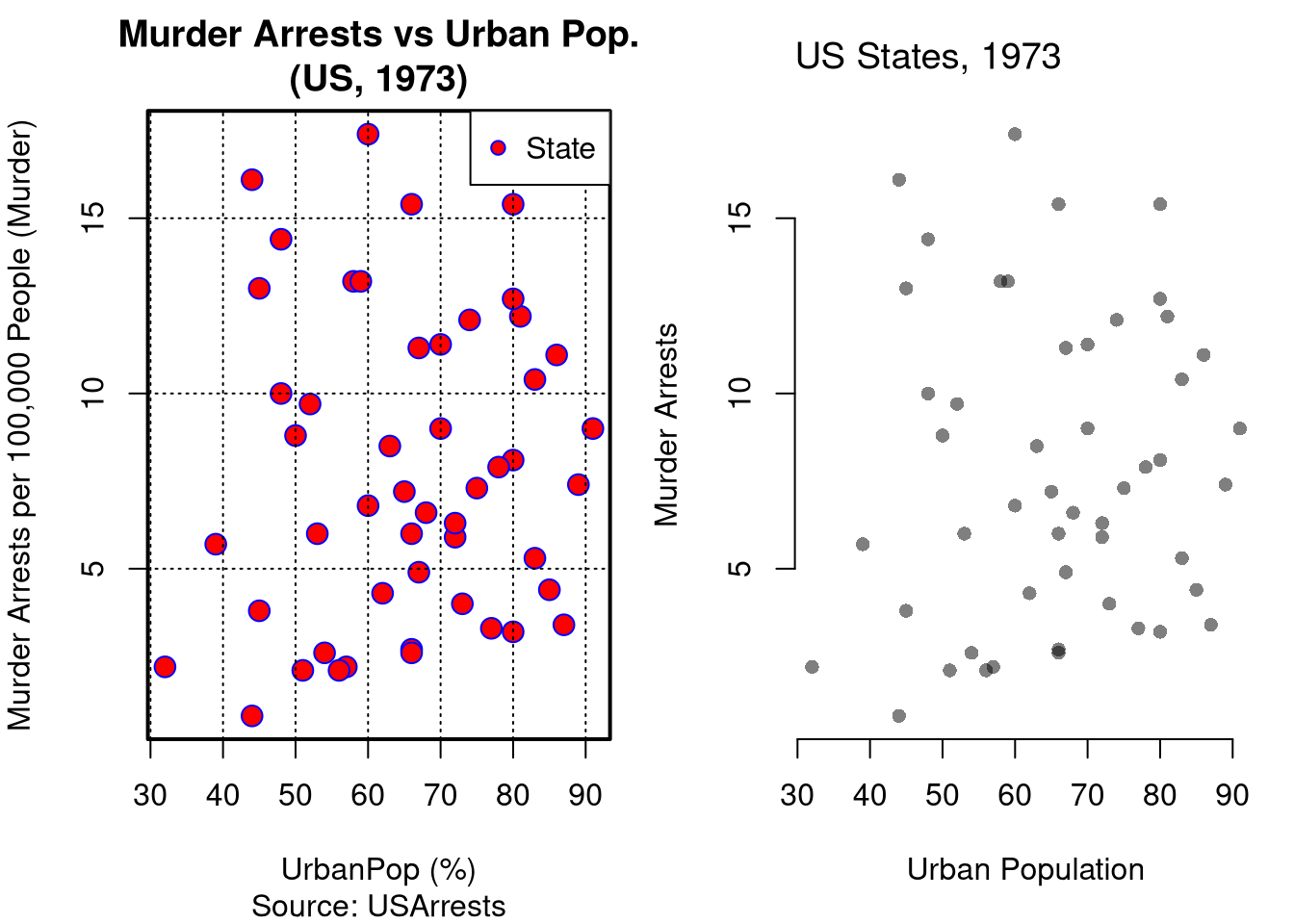
Repeat the comparison with USArrests, a much smaller dataset. Does the cluttered panel still hide any points?

# 50 US states, 1973
xy2_hat <- USArrests[, c('UrbanPop', 'Murder')]
colnames(xy2_hat) <- c('x_hat', 'y_hat') # x_hat=urban population share, y_hat=murder arrests per 100K

par(mfrow=c(1, 2), mar=c(5, 4, 3, 1))

# Cluttered: oversized two-color markers, gridlines, redundant title
plot(y_hat ~ x_hat, data=xy2_hat,
    pch=21, bg='red', col='blue', cex=1.5,
    main='Murder Arrests vs Urban Pop.\n(US, 1973)',
    sub='Source: USArrests',
    xlab='UrbanPop (%)',
    ylab='Murder Arrests per 100,000 People (Murder)')
grid(col='black', lwd=1)
box(lwd=2)
legend('topright', legend='State', pch=21, pt.bg='red', col='blue')

# Polished: light points, no grid, no redundant labels or legend
plot(y_hat ~ x_hat, data=xy2_hat,
    pch=16, col=grey(0, .5),                     # transparent black points
    main=NA, xlab='Urban Population', ylab='Murder Arrests',
    bty='n')                                     # drop the surrounding box
title('US States, 1973', font.main=1, adj=0)

# Both panels show a very weak positive relationship across the 50 states.
# With so few points, the markers barely overlap.
# So both panels carry the same information about the data.

TipTest Yourself

A colleague sends a scatterplot of monthly sales against advertising spend. It has a shaded background, a drop-shadow on every point, a 3D tilt, a legend that names the single series “Series 1”, and a company logo in the corner. Which elements should you remove, and what (if anything) should you add?

The shading, drop-shadows, 3D tilt, one-entry legend, and logo are all non-data ink: none of them help a reader read sales against spend, so all can go. Keep the points and clear axis labels. If a few months are special (say, a promotion), a short text label on those points is necessary ink worth adding.

NoteMust Know

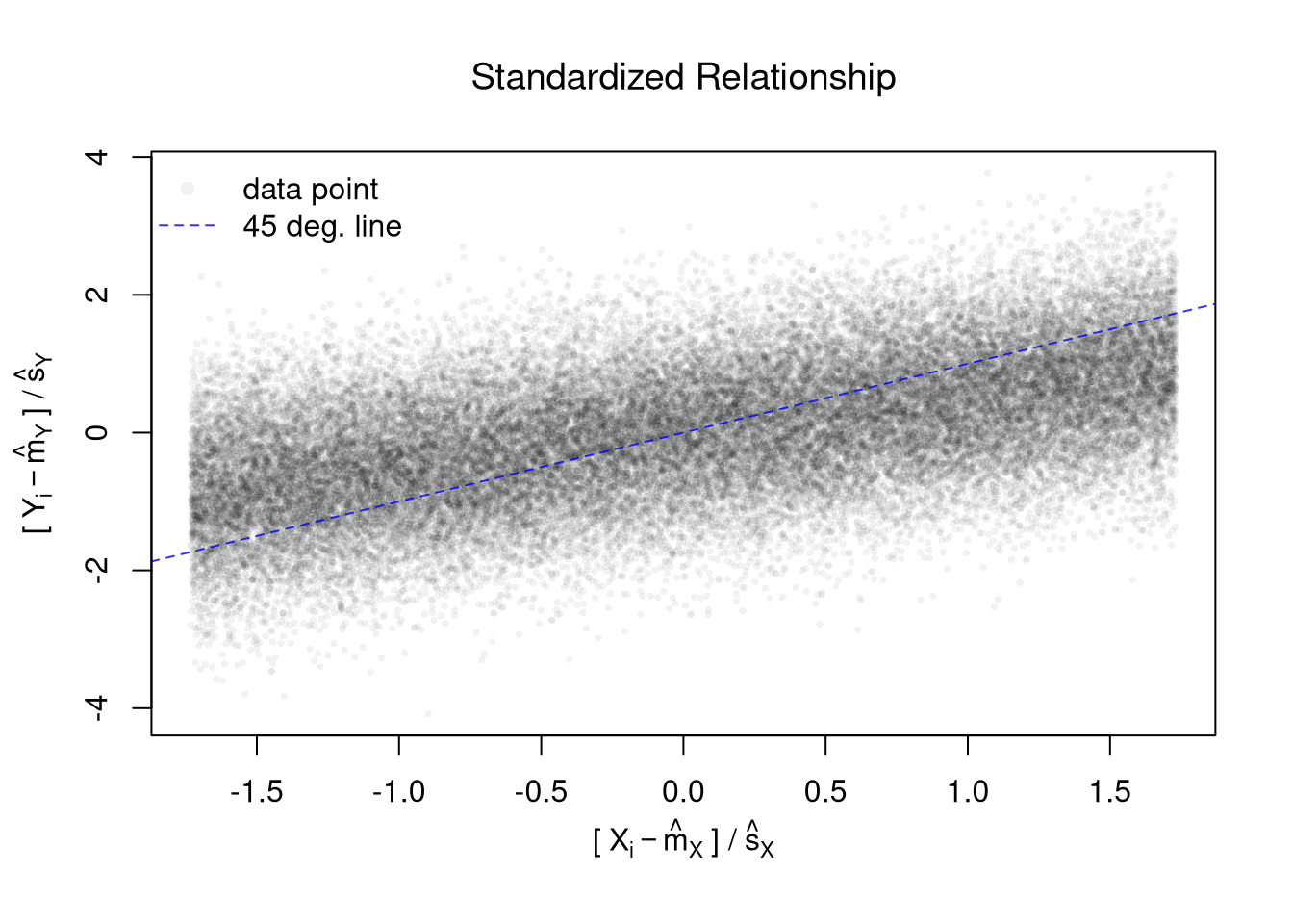
Polishing a plot with many points. The simulated data below have tens of thousands of points, so a default first draft would be a solid black blob. The second draft standardizes both variables, uses small transparent points, and adds a 45 degree line for reference.

# Random Data: 45,001 points
x_sim <- seq(1, 10, by=.0002)
e <- rnorm(length(x_sim), mean=0, sd=1)
y_sim <- .25*x_sim + e

# First Draft
# plot(x_sim, y_sim)

# Second Draft: Focus
# (In this example: relationship magnitude)
x_std_sim <- scale(x_sim)
y_std_sim <- scale(y_sim)
plot(x_std_sim, y_std_sim,
    xlab='', ylab='',
    pch=16, cex=.5, col=grey(0, .05),
    main=NA)
mtext(expression('['~X[i]-hat(m)[X]~'] /'~hat(s)[X]), 1, line=2.5)
mtext(expression('['~Y[i]-hat(m)[Y]~'] /'~hat(s)[Y]), 2, line=2.5)
# Add a 45 degree line
abline(a=0, b=1, col=rgb(0, 0, 1, .8), lty=2)
legend('topleft',
    legend=c('data point', '45 deg. line'),
    pch=c(16, NA), lty=c(NA, 2), col=c(grey(0, .05), rgb(0, 0, 1, .8)),
    bty='n')
title('Standardized Relationship', font.main=1)

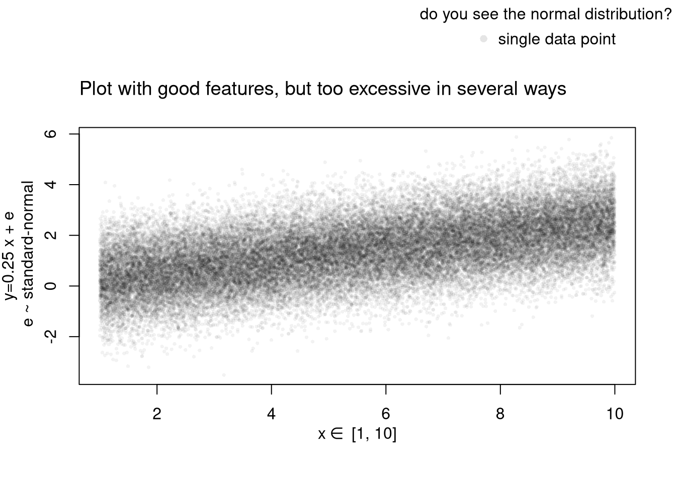
The next version of the same data has good features, but goes too far. The math in the axis labels, the outer legend, and the long title all add ink the reader does not need.

# Another Example
xy_sim <- data.frame(x_sim=x_sim, y_sim=y_sim)
par(fig=c(0, 1, 0, 0.9), new=FALSE)
plot(y_sim ~ x_sim, xy_sim, pch=16, col=grey(0, .05), cex=.5,
    main=NA, xlab='', ylab='') # Format Axis Labels Separately
mtext( 'y=0.25 x + e\n e ~ standard-normal', 2, line=2.2)
mtext( expression(x%in%~'[1, 10]'), 1, line=2.2)
#abline( lm(y_sim ~ x_sim, data=xy_sim), lty=2)
title('Plot with good features, but too excessive in several ways',
    adj=0, font.main=1)

# Outer Legend (https://stackoverflow.com/questions/3932038/)
outer_legend <- function(...) {
  opar <- par(fig=c(0, 1, 0, 1), oma=c(0, 0, 0, 0), 
    mar=c(0, 0, 0, 0), new=TRUE)
  on.exit(par(opar))
  plot(0, 0, type='n', bty='n', xaxt='n', yaxt='n')
  legend(...)
}
outer_legend('topright', legend='single data point',
    title='do you see the normal distribution?',
    pch=16, col=rgb(0, 0, 0, .1), cex=1, bty='n')

Learn to edit your figures:

• https://socviz.co/08-polishing.html – K. Healy’s chapter on refining a draft figure with color, annotation, and themes (its code uses ggplot2).
• https://websites.umich.edu/~jpboyd/eng403_chap2_tuftegospel.pdf
• https://jtr13.github.io/cc19/tuftes-principles-of-data-ink.html
• https://github.com/cxli233/FriendsDontLetFriends
• https://www.edwardtufte.com/notebook/chartjunk/
• https://www.biostat.wisc.edu/~kbroman/topten_worstgraphs/
• https://www.businessinsider.com/the-27-worst-charts-of-all-time-2013-6

Which features are most informative depends on what you want to show, and you can always mix and match. Be aware that each type has benefits and costs. E.g., see

• https://www.data-to-viz.com/caveats.html
• https://x.com/EdwardTufte/status/1092717905156993024/photo/1
• Hintze and Nelson (1998) – why a boxplot alone can hide the distribution’s shape, and what to pair it with.

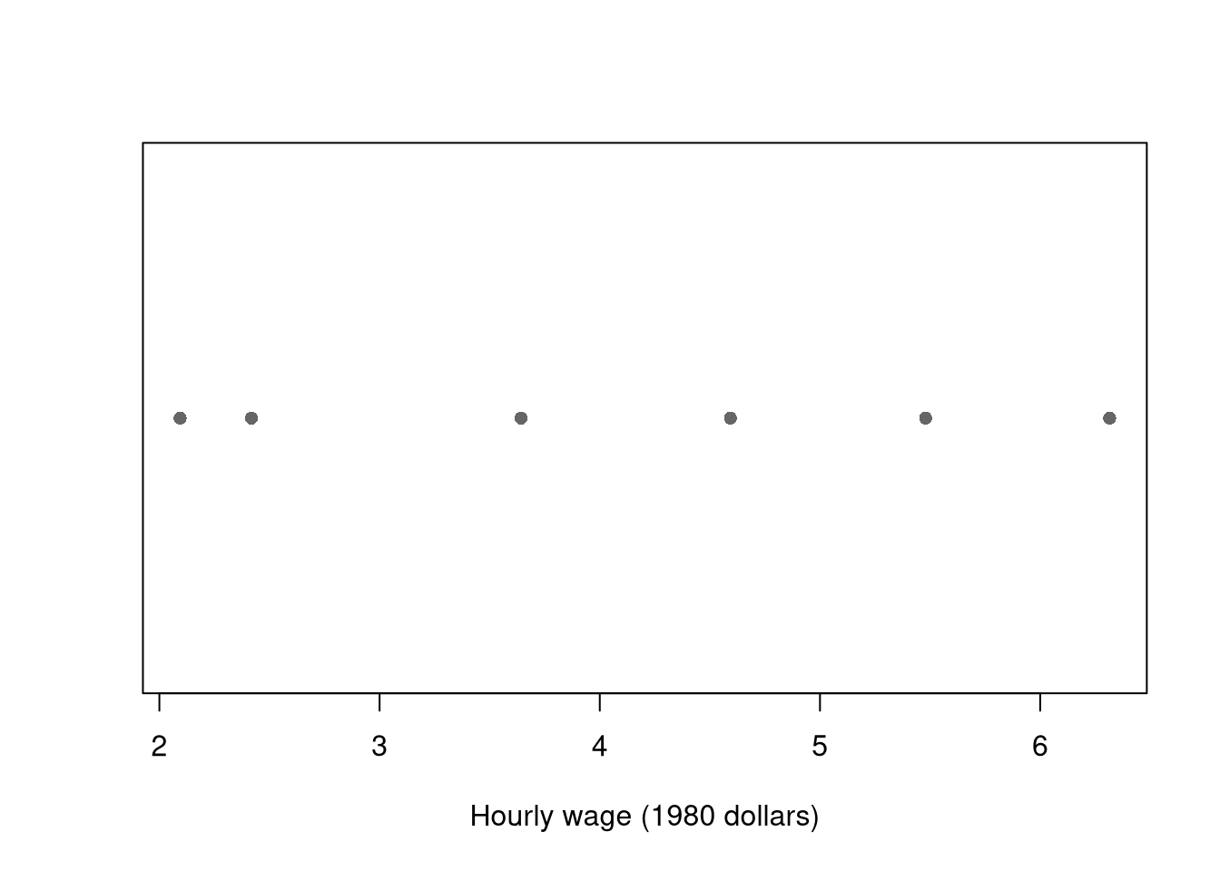
For small datasets, you can plot individual data points with a strip chart.

NoteMust Know

A strip chart shows every observation as a point along one axis, which works well when there are too few points to justify a histogram or boxplot.

# Six workers: show each hourly wage directly
y_small_hat <- xy_hat[1:6, 'y_hat']
stripchart(y_small_hat, pch=16, col=grey(0, .6),
    xlab='Hourly wage (1980 dollars)')

With few values, a strip chart shows the data honestly; a boxplot would hide the individual points behind summary statistics.

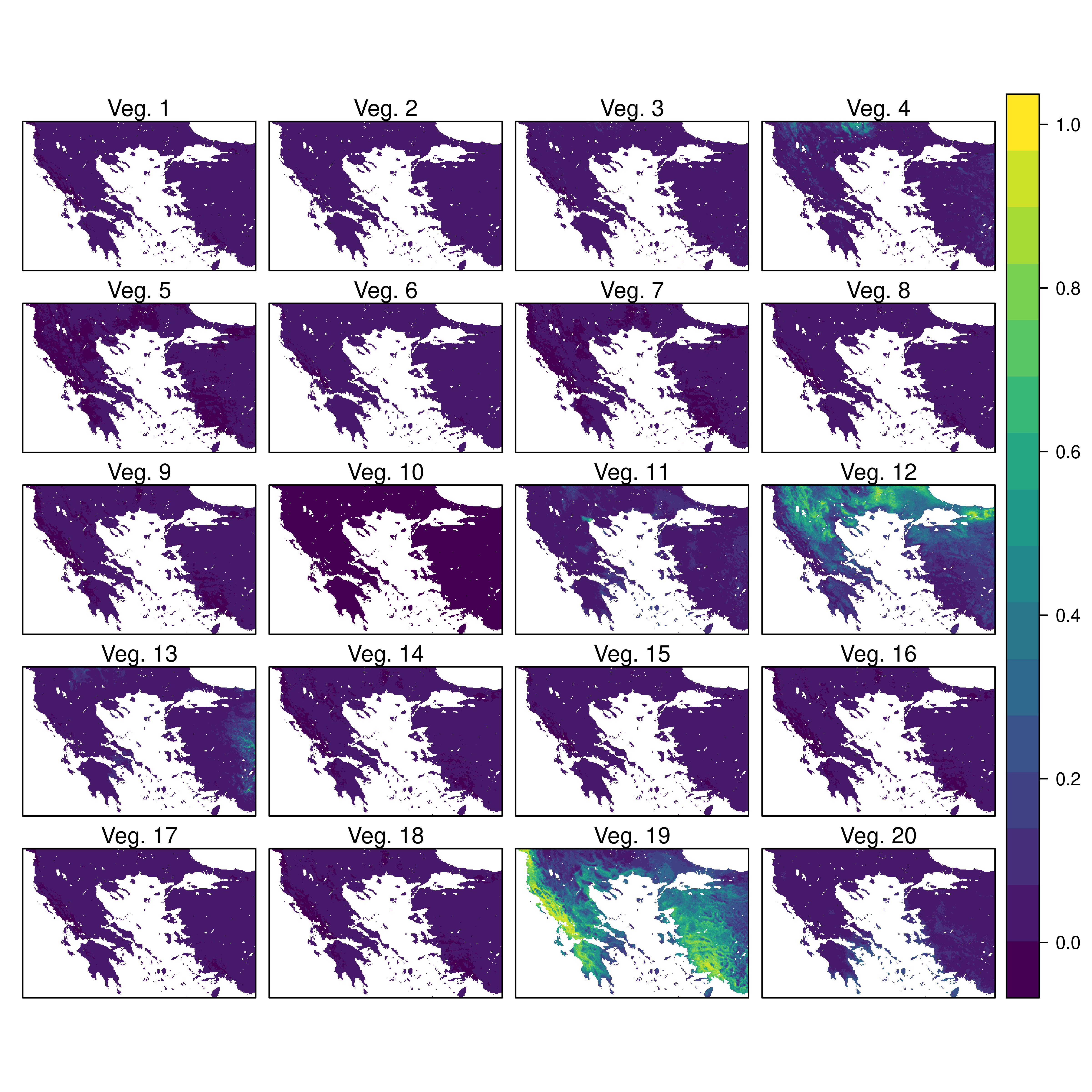
For datasets with spatial information, a map is also helpful. Sometimes tables are better than graphs (see https://www.edwardtufte.com/notebook/boxplots-data-test). For useful tips, see C. Wilke (2019) “Fundamentals of Data Visualization: A Primer on Making Informative and Compelling Figures” https://clauswilke.com/dataviz/.

For plotting math, which should be done very sparingly, see https://astrostatistics.psu.edu/su07/R/html/grDevices/html/plotmath.html and https://library.virginia.edu/data/articles/mathematical-annotation-in-r.

Static Publishing

NoteMust Know

You can export figures with specific dimensions

pdf( 'Figures/plot_example.pdf', height=5, width=5)
# plot goes here
dev.off()

For exporting options, see ?pdf. For saving other types of files, see png("*.png"), tiff("*.tiff"), and jpeg("*.jpg")

You can also export tables in a variety of formats, including many that other software programs can easily read

library('stargazer')
# summary statistics
stargazer(Wages1,
    type='html',
    summary=TRUE,
    title='Summary Statistics for Wages1')

Summary Statistics for Wages1

Statistic	N	Mean	St. Dev.	Min	Max
exper	3,294	8.043	2.291	1	18
school	3,294	11.631	1.658	3	16
wage	3,294	5.758	3.269	0.077	39.809

# The table covers the numeric columns only, so the factor sex is left out.

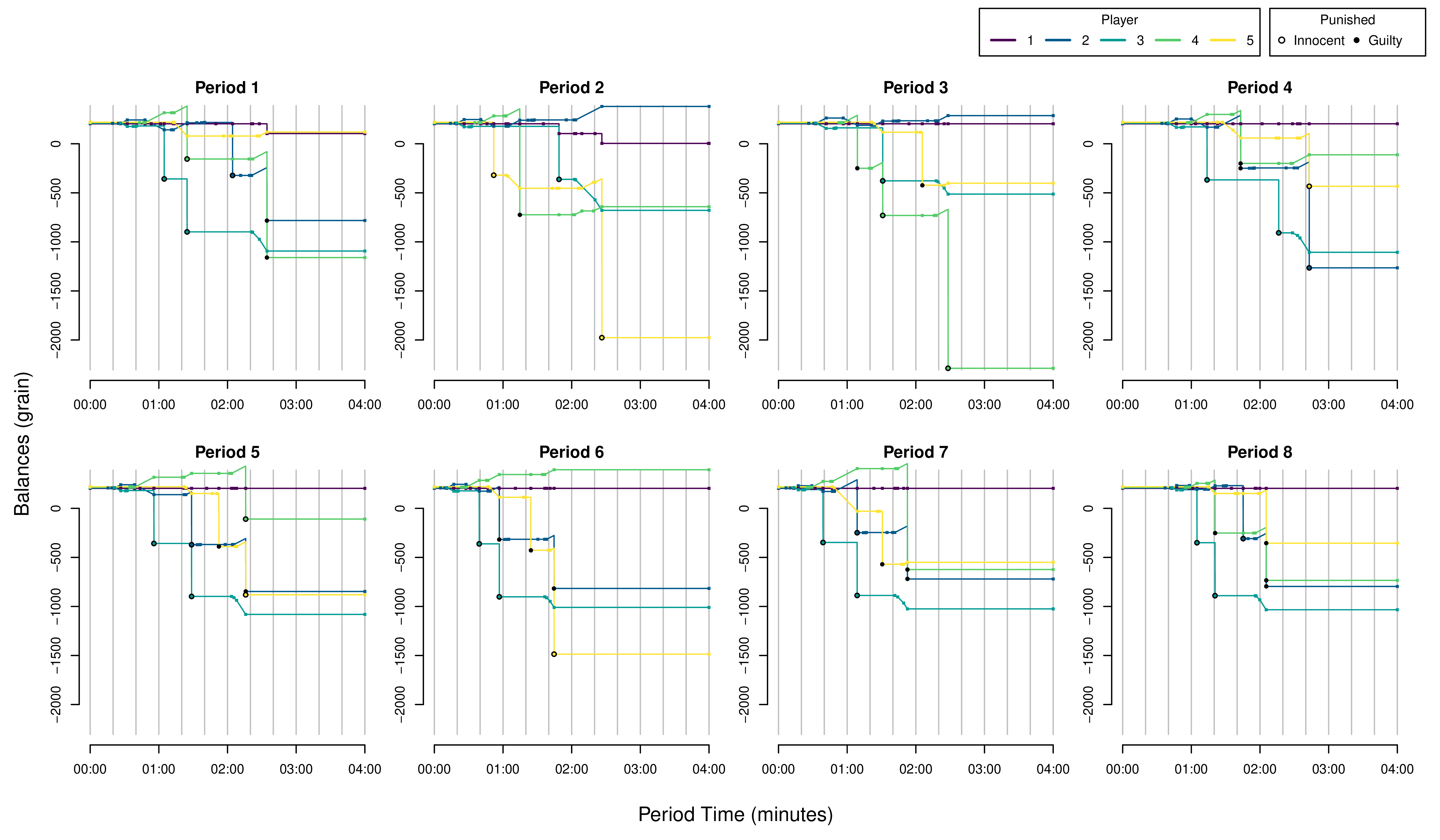
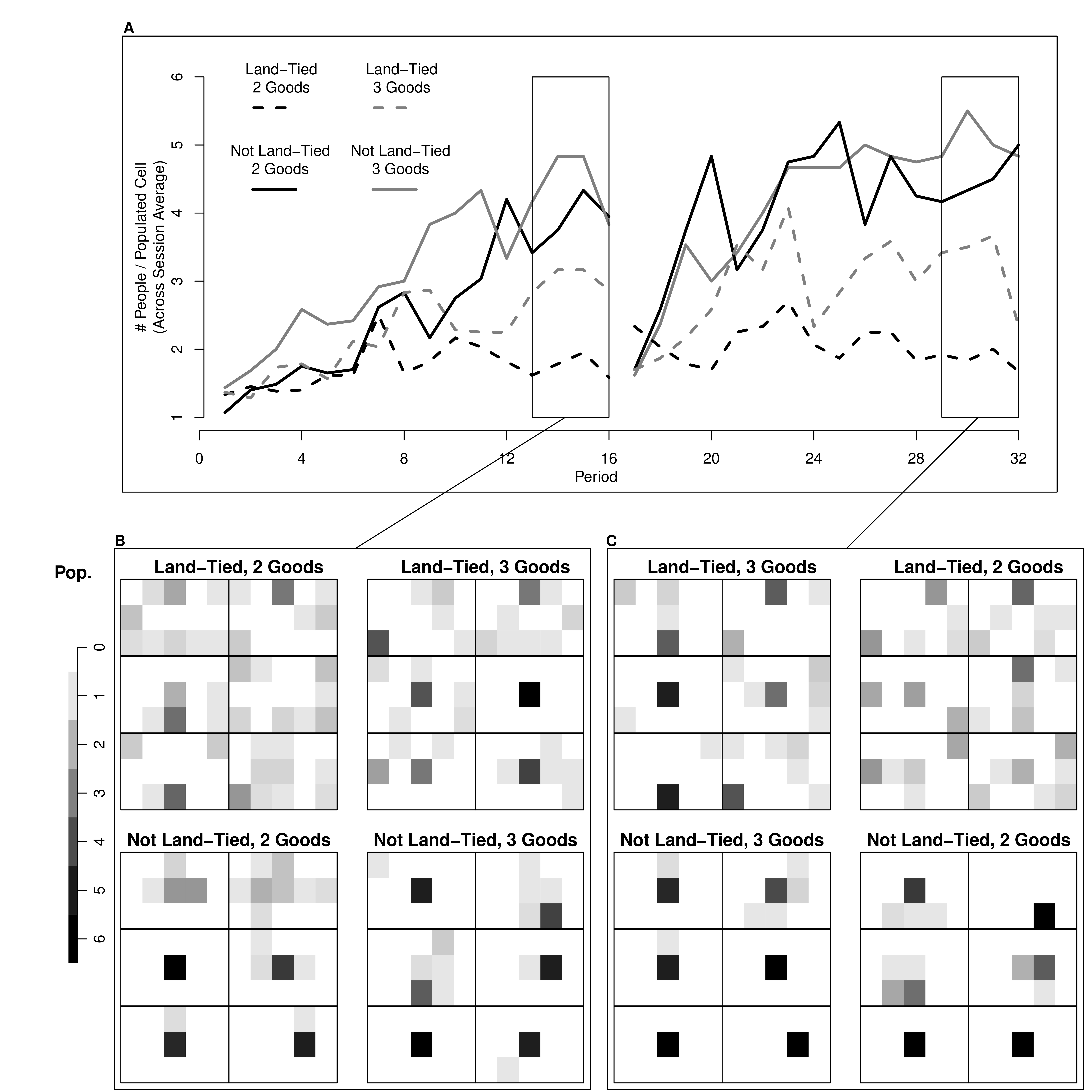
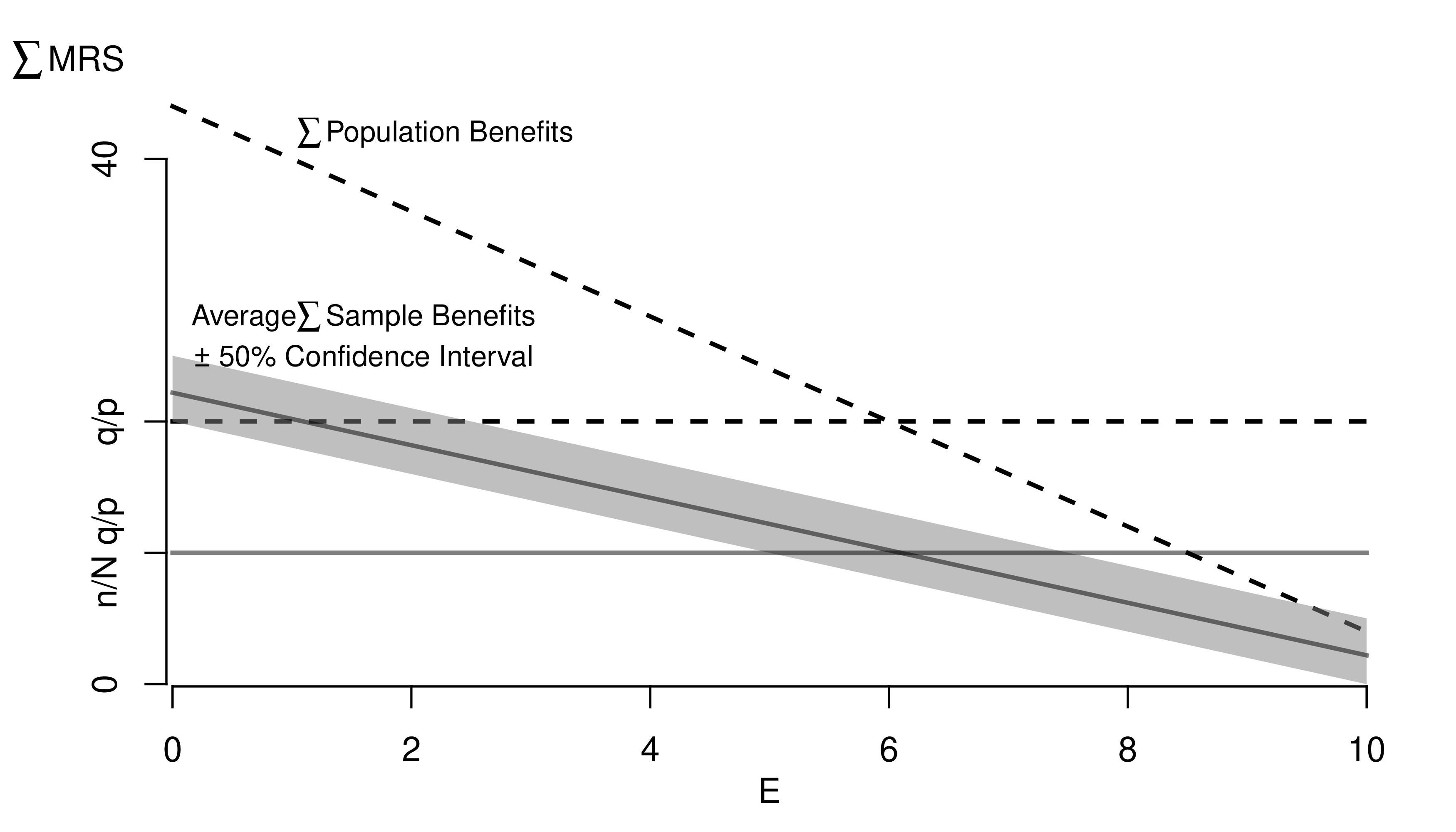
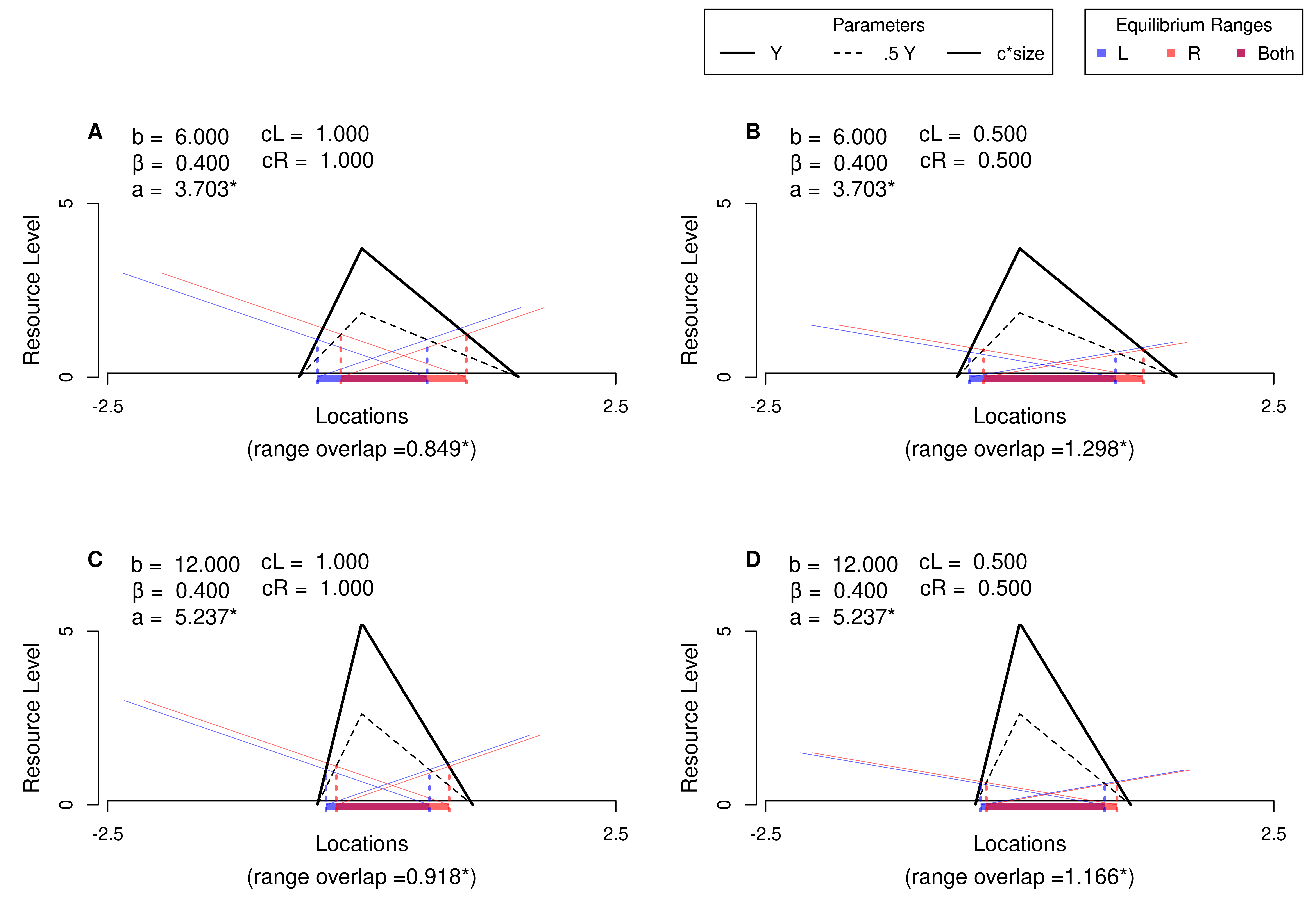
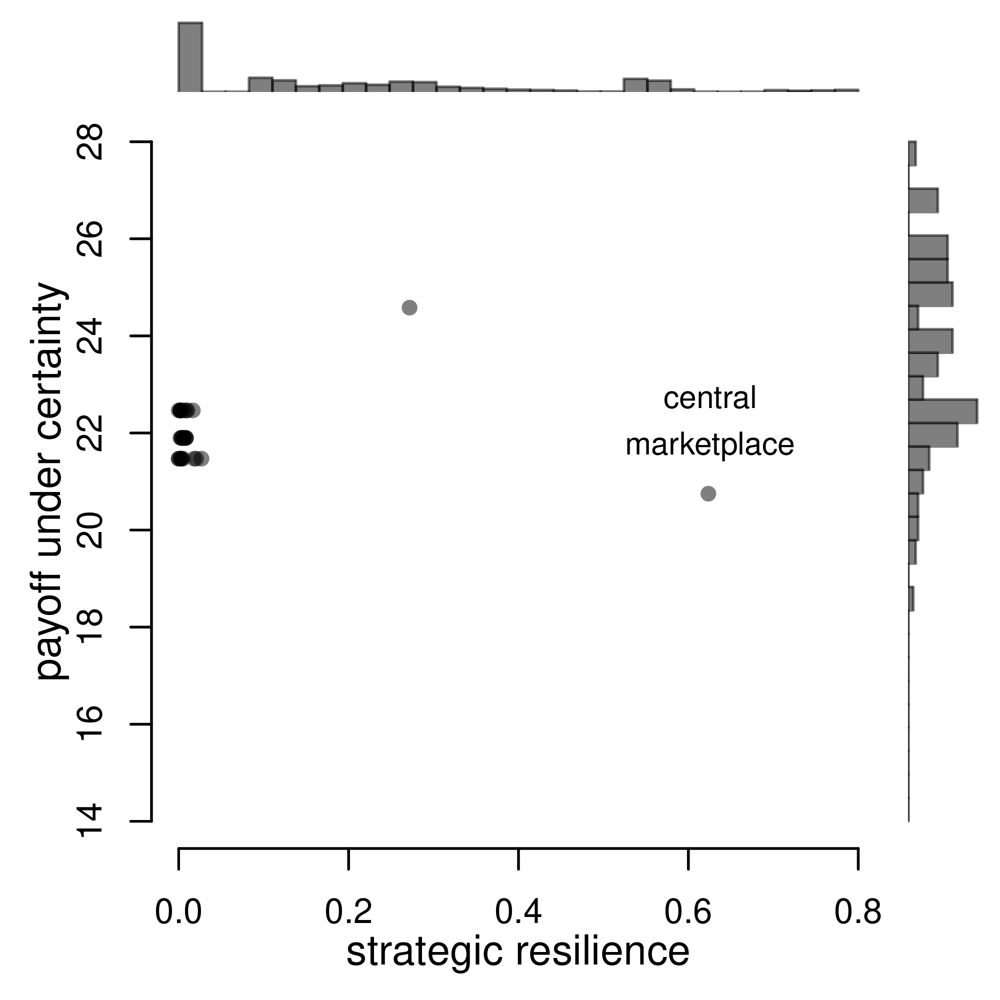
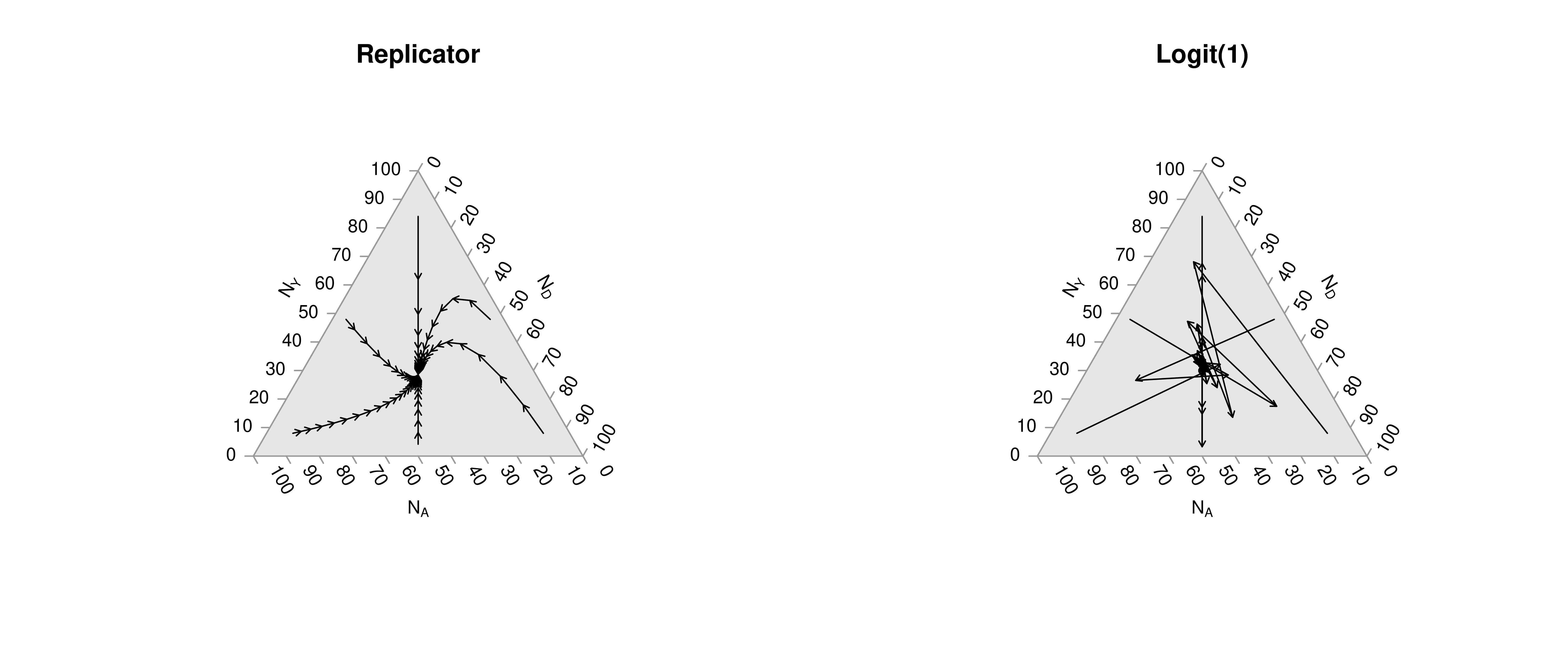
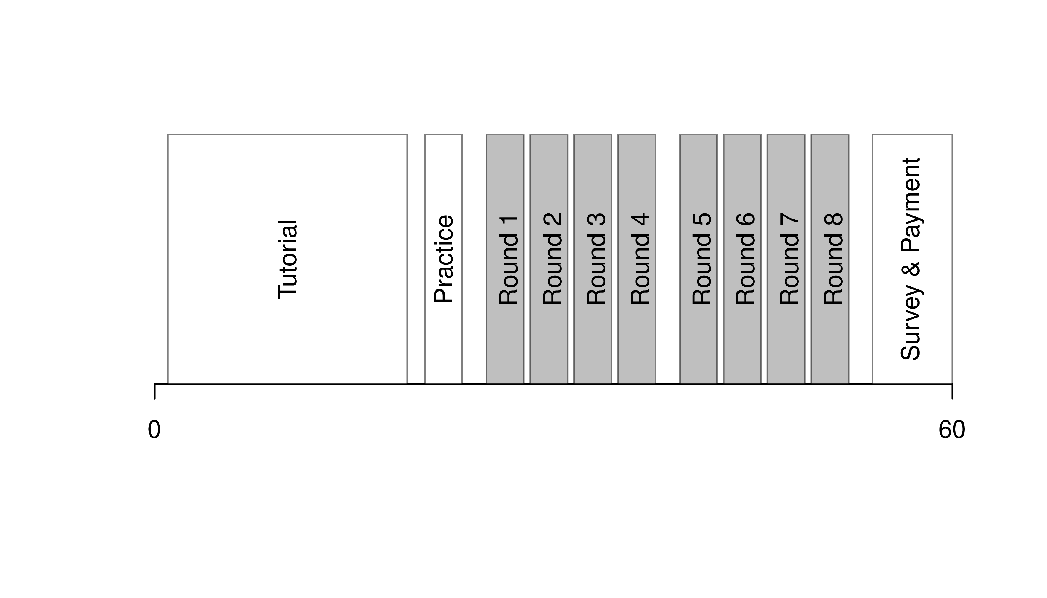
Note that many of the best plots are custom made (see https://www.r-graph-gallery.com/). Here are some ones that I have made over the years.

20.2 Quarto Reports

Quarto Documents

A statistical analysis usually has code that produces numbers and prose that explains them. Keeping the two in sync by hand is the source of most reproducibility failures. A Quarto document (.qmd file) is a plain-text source that interleaves prose with executable R code chunks. Rendering produces a self-contained output (HTML, PDF, or Word) where the code, its results, and the surrounding text all stay in sync.

Quarto is useful as the format for any analysis that has both writing and computation: homework reports, technical notes, papers, slides, and the chapters of this book. R does the statistical computation and Quarto formats those computations into a polished document. Altogether, your project will use

• R: does statistical computations
• Quarto: formats statistical computations for sharing (.qmd files)
• RStudio: graphical user interface that allows you to easily use both R and Quarto

Reproducible Reports

Quarto handles the mechanics of mixing code and prose, which is one step toward a reproducible report.

ImportantKey Definition

A reproducible report is one whose final figures, tables, and numbers can be regenerated from the source file alone, by anyone with the data and the listed software versions.

Reproducible reports are useful because they let collaborators (and your future self) re-run the analysis after data are updated, methods are corrected, or a coauthor wants to check a number. Published research applies the same idea with a public replication package (Peng 2011; Christensen and Miguel 2018). Homework reports are the smallest version of this: simple reproducible reports that are almost entirely self-contained (showing both code and output). To make them, you need Quarto installed on your computer.

• RStudio (version 2022.07 or later) includes Quarto

Example

Start by opening RStudio, then

• Click “File > New File > Quarto Document”
• Add your name and a title
• Save the file as “COURSEID_Template_Lastname.qmd”
• Click “Render”
• Notice how the code in the source document corresponds to formatting in the output document

Now try each of the following steps, re-rendering the document after each step

• Basic Formatting:
  • Change the title to “My First Quarto Document”
  • Change the bold word Render to italics: Render
  • Create a new section header at the bottom called “Data Analysis”
• Data Analysis:
  • Make a simple scatterplot for Murder vs. UrbanPop in the USArrests data
  • Change the simple scatterplot into a polished interactive scatterplot
  • Before the scatterplot add a reactable table for the raw data
  • Write your own description of a) the dataset and b) the relationship between Murder and UrbanPop
• Polishing
  • Delete the default sections
  • clean up your analysis (make sure the table,figure, and writing are high quality)
  • Email the output, “COURSEID_Template_Lastname.html”, to yourself

20.3 Exercises

1. Comment the script you wrote for this chapter, then restart R and check that it runs from a clean session, then check the script with AI as explained in Working with AI. Write three sentences from memory on the main statistical idea of this chapter, and ask the assistant what is wrong, vague, or missing. Finish with your own questions about whatever you found hardest.

2. When polishing a figure, you must both add necessary details and remove unnecessary ones. Give one example of each for a scatterplot of Murder vs. UrbanPop in the USArrests dataset.

3. Using the USArrests dataset, compute summary statistics (mean, standard deviation, min, max) for all four variables. Present the results in a single data frame with one row per variable.

4. Using the USArrests dataset and the plotly library, write R code to create an interactive scatterplot of Murder (y-axis) vs. UrbanPop (x-axis). The hover text should display the state name, murder rate, and urban population percentage.

Further Reading

• https://quarto.org/docs/guide/ – the official Quarto guide, covering document types, code cells, and output formats.
• https://r4ds.hadley.nz/quarto – practical chapter on integrating Quarto into a data-analysis workflow.
• https://rstudio.github.io/cheatsheets/quarto.pdf – two-page cheat sheet for quick reference on cell options and formatting syntax.

Recall

This chapter covered interactive figures and tables, the data-ink ratio, and Quarto for reproducible reports. Most examples used the Wages1 data. A plotly scatterplot showed each worker’s sex, schooling, and wage as hover text, and a reactable table showed summary statistics. Side-by-side panels compared a cluttered and a polished scatterplot of wage vs. school.

Christensen, Garret, and Edward Miguel. 2018. “Transparency, Reproducibility, and the Credibility of Economics Research.” Journal of Economic Literature 56 (3): 920–80. https://doi.org/10.1257/jel.20171350.

Hintze, Jerry L., and Ray D. Nelson. 1998. “Violin Plots: A Box Plot-Density Trace Synergism.” The American Statistician 52 (2): 181–84. https://doi.org/10.1080/00031305.1998.10480559.

Peng, Roger D. 2011. “Reproducible Research in Computational Science.” Science 334 (6060): 1226–27. https://doi.org/10.1126/science.1213847.

Tufte, Edward. 2001. The Visual Display of Quantitative Information. 2nd ed. Graphics Press. https://www.google.de/books/edition/The_Visual_Display_of_Quantitative_Infor/qmjNngEACAAJ.