19  Classical Tests and Bias-Variance

---

Earlier chapters tested hypotheses with resampling.

This chapter asks two questions.

• Can we test hypotheses with formulas instead of resampling?
  • Welch’s \(t\)-test and the \(z\)-statistic: these divide a difference in means by its standard error, as the \(t\)-value did for one mean. When the data are well-behaved, the sampling distribution of this ratio is known in advance, so a formula gives the \(p\)-value.
  • \(t\)-statistic for a slope: this applies the same ratio to the regression slope, \(\hat{t}=\hat{b}_{1}/\hat{\text{SE}}(B_{1})\).
  • \(z\)-statistic for a difference in medians: this forms the same ratio from the standard errors behind R’s default boxplot notches.
• How do regression estimates miss their target?
  • Bias-variance tradeoff: with the conditional expectation as the target, this splits prediction error into squared bias and variance. Cutting one piece usually raises the other.
  • Consistency: this property needs both pieces to shrink as \(n\) grows. For local regression, that works if the bandwidth also shrinks, but not too fast.

19.1 Classical Tests

Just as with one sample tests, we can compute standardized differences. The observed difference is converted into a \(t\)-statistic by dividing by an estimated standard error. Note, however, that we have to compute the standard error for the difference statistic, which is a bit more complicated than for a single sample. Under the assumption that both populations are independently distributed, we can analytically derive the sampling distribution for the differences between two groups.

Differences in Means

Let \(Y_{ig}\) denote the random outcome for individual \(i\) in group \(g\). To compare two group means, we standardize the observed difference by its estimated standard error.

ImportantKey Definition

The two-sample t-statistic divides the observed mean difference by its estimated standard error: \[\hat{t} = \frac{\hat{m}_{1} - \hat{m}_{2}}{\sqrt{\hat{s}^2_{1,\text{adj}}/n_{1}+\hat{s}^2_{2,\text{adj}}/n_{2}}},\] where \(\hat{s}^2_{g,\text{adj}}\) is the adjusted sample variance and \(n_{g}\) is the sample size for group \(g\).

Welch’s t-test (Welch 1947) modifies the two-sample \(\hat{t}\) above to account for unequal variances or unequal sample sizes. The modifications use the Welch-Satterthwaite approximation.

The two-sample \(\hat{t}\) is useful as a standardized test statistic for comparing two means. Dividing by the standard error puts the gap in standard-error units. So the same numerator can be large or small in \(\hat{t}\) units, depending on \(n_{1}, n_{2}\) and the within-group variances. With normally distributed data in each group, this statistic follows Student’s t-distribution (Student 1908), so we can read a \(p\)-value from a formula rather than from resampling. When the two groups have unequal variances or sample sizes, a small adjustment to the degrees of freedom keeps the \(t\)-distribution approximation accurate.

The \(t\)-distribution result needs normal data, but in large samples the central limit theorem makes the difference in means approximately normal whatever the shape of the data.

ImportantKey Definition

The \(z\)-statistic standardizes an estimate by its estimated standard error, as \(\hat{t}\) does, but compares the result to the standard normal rather than to a \(t\)-distribution. For the difference statistic \(\hat{d}\) and the null of no difference, \[\hat{z} = \frac{\hat{d}}{\hat{\text{SE}}(D)}.\]

The \(z\)-statistic is useful because it only needs the estimate to be approximately normal, which holds in large samples for many statistics besides the mean. For means, \(\hat{d}=\hat{m}_{1}-\hat{m}_{2}\) and \(\hat{\text{SE}}(D)=\sqrt{\hat{s}^2_{1,\text{adj}}/n_{1}+\hat{s}^2_{2,\text{adj}}/n_{2}}\), so \(\hat{z}\) is the same number as the two-sample \(\hat{t}\); only the reference distribution changes. The two-sided \(p\)-value is the probability that a standard normal draw lands at least \(|\hat{z}|\) from zero, which R computes as 2 * pnorm(-abs(z_hat)). The standard normal has thinner tails than any \(t\)-distribution, so the \(z\) \(p\)-value is smaller, but the gap shrinks as the groups grow.

For example, the code below compares two group means with Welch’s \(t\)-test.

## MAIN EXAMPLE
# Hourly wages in 1980 dollars for 3294 US workers
data(Wages1, package='Ecdat')
# The levels are in this order, so the reported difference is female minus male
levels(Wages1[, 'sex'])
## [1] "female" "male"

# Welch's t-test (the default for t.test)
t.test(wage ~ sex, data=Wages1)
## 
##  Welch Two Sample t-test
## 
## data:  wage by sex
## t = -10.485, df = 3259.3, p-value < 2.2e-16
## alternative hypothesis: true difference in means between group female and group male is not equal to 0
## 95 percent confidence interval:
##  -1.384162 -0.948033
## sample estimates:
## mean in group female   mean in group male 
##             5.146924             6.313021
# The female mean is about 1.17 dollars below the male mean.
# The reported t is also the z-statistic, about -10.5.
# With more than 1500 workers per group, both p-values are essentially zero.

NoteMust Know

The same test works on simulated data, where we choose the group means ourselves. Here the two groups have different means and different variances.

# Sample 1
n1 <- 100
y1_sim <- rnorm(n1, 0, 2)
#hist(y1_sim, freq=FALSE, main='Sample 1')

# Sample 2
n2 <- 80
y2_sim <- rnorm(n2, 1, 1)
#hist(y2_sim, freq=FALSE, main='Sample 2')

t.test(y1_sim, y2_sim, var.equal=FALSE)
## 
##  Welch Two Sample t-test
## 
## data:  y1_sim and y2_sim
## t = -3.6939, df = 158.27, p-value = 0.0003037
## alternative hypothesis: true difference in means is not equal to 0
## 95 percent confidence interval:
##  -1.190604 -0.360992
## sample estimates:
## mean of x mean of y 
## 0.2177747 0.9935727

Welch’s \(t\)-test is useful as the default for comparing two means without assuming equal variances. Unequal variances are common in applied work, for example when comparing two job markets or two countries. With the variance-and-normality assumptions in place, the test can be conducted entirely with formulas (no bootstrap resampling required). Compare the bootstrap test of a mean difference in Two Groups, which needed neither assumption.

NoteMust Know

The Welch-Satterthwaite equation (Satterthwaite 1946; Welch 1947) approximates the degrees of freedom when the two groups have unequal variances: \[ \text{df} = \frac{\left(\hat{s}^2_{1,\text{adj}}/n_{1} + \hat{s}^2_{2,\text{adj}}/n_{2}\right)^2}{\frac{(\hat{s}^2_{1,\text{adj}}/n_{1})^2}{n_{1}-1} + \frac{(\hat{s}^2_{2,\text{adj}}/n_{2})^2}{n_{2}-1}}. \] For example, suppose both groups have \(n_{1}=n_{2}=10\), with adjusted sample variances \(\hat{s}^2_{1,\text{adj}}=4\) and \(\hat{s}^2_{2,\text{adj}}=1\). Writing \(v_{g}=\hat{s}^2_{g,\text{adj}}/n_{g}\), we have \(v_{1}=0.4\) and \(v_{2}=0.1\), so \[ \text{df} = \frac{(0.4+0.1)^2}{0.4^2/9 + 0.1^2/9} = \frac{0.25}{0.17/9} \approx 13.2. \] This is below the equal-variance value \(n_{1}+n_{2}-2=18\): unequal variances cost degrees of freedom, which widens the \(t\)-distribution and makes the test more conservative.

n01 <- 10; n02 <- 10
v01_hat <- 4/n01
v02_hat <- 1/n02
(v01_hat + v02_hat)^2 / (v01_hat^2/(n01-1) + v02_hat^2/(n02-1))
## [1] 13.23529

NoteMust Know

Continue the Welch-Satterthwaite example, with \(n_{1}=n_{2}=10\), \(\hat{s}^2_{1,\text{adj}}=4\), and \(\hat{s}^2_{2,\text{adj}}=1\), and suppose \(\hat{d}=\hat{m}_{1}-\hat{m}_{2}=1.5\). Then \(\hat{\text{SE}}(D)=\sqrt{0.4+0.1}=\sqrt{0.5}\approx 0.71\), so \(\hat{z}=\hat{t}=1.5/\sqrt{0.5}\approx 2.12\). The standard normal gives a \(p\)-value of about \(0.034\), while the \(t\)-distribution with \(13.2\) degrees of freedom gives about \(0.053\). With only \(10\) observations per group, the two reference distributions disagree about rejecting at the \(5\%\) level.

# The two groups from the Welch-Satterthwaite example, with a mean difference of 1.5
d0_hat <- 1.5
se0_hat <- sqrt(v01_hat + v02_hat)
z0_hat <- d0_hat / se0_hat # the same number as the two-sample t-statistic
df0 <- (v01_hat + v02_hat)^2 / (v01_hat^2/(n01 - 1) + v02_hat^2/(n02 - 1))

# Same statistic, two reference distributions
c(z=z0_hat,
    p_normal=2 * pnorm(-abs(z0_hat)),
    p_t=2 * pt(-abs(z0_hat), df=df0))
##          z   p_normal        p_t 
## 2.12132034 0.03389485 0.05332678

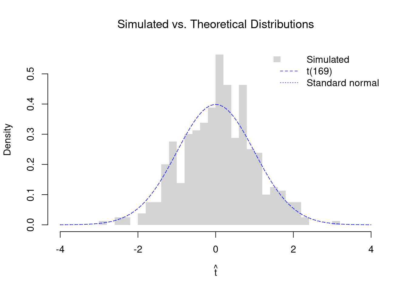
We can visualize this by simulating many samples under the null (\(\mathbb{E}[Y_{i1}]=\mathbb{E}[Y_{i2}]\)) and comparing the distribution of \(\hat{t}\) with the theoretical \(t\)-distribution (dashed curve) and the standard normal used for \(\hat{z}\) (dotted curve). As in Sampling, pretend the data are the whole population. If we draw both groups from the same population, then the null of equal means holds exactly.

# Pretend these 3294 workers are the whole population
data(Wages1, package='Ecdat')
population_xy <- Wages1[, c('school', 'wage')]
colnames(population_xy) <- c('x', 'y') # x=years of schooling, y=hourly wage
population_wages <- population_xy[, 'y']

# Simulate the t-statistic under the null (both groups from the same population)
n1 <- 100
n2 <- 80
n_sim <- 399
t_sim <- vector(length = n_sim)
for (b in seq(n_sim)) {
    y1_sim_b <- population_wages[sample(length(population_wages), n1, replace=FALSE)]
    y2_sim_b <- population_wages[sample(length(population_wages), n2, replace=FALSE)]
    t_sim[b] <- t.test(y1_sim_b, y2_sim_b, var.equal = FALSE)$statistic
}

# Welch-Satterthwaite degrees of freedom
# (use the population variance for both groups)
v1 <- var(population_wages) / n1
v2 <- var(population_wages) / n2
df_ws <- (v1 + v2)^2 / (v1^2 / (n1 - 1) + v2^2 / (n2 - 1))

# Overlay: simulated histogram vs. theoretical t-distribution
t_range <- range(c(t_sim, -4, 4))
hist(t_sim, breaks = 30, freq = FALSE, border = NA,
    xlim = t_range,
    xlab = expression(hat(t)),
    main = NA)
title('Simulated vs. Theoretical Distributions', font.main = 1)
t_grid <- seq(t_range[1], t_range[2], length = 200)
lines(t_grid, dt(t_grid, df = df_ws), col = rgb(0, 0, 1, .8), lty = 2)
lines(t_grid, dnorm(t_grid), col = rgb(0, 0, 1, .8), lty = 3) # standard normal, for z
legend('topright', legend = c('Simulated', paste0('t(', round(df_ws), ')'), 'Standard normal'),
    fill = c(grey(.83), NA, NA), border = NA, # grey(.83) matches the default histogram fill
    lwd = c(NA, 1, 1), lty = c(NA, 2, 3), col = c(NA, rgb(0, 0, 1, .8), rgb(0, 0, 1, .8)), bty = 'n')

# Wages are right-skewed, so the group means are not exactly normal.
# With groups of 100 and 80, the histogram is typically close to both curves.
# The curves nearly coincide because t has about 170 degrees of freedom here.
# So z gives almost the same p-value as t.

When the data are skewed, the group means are not exactly normal and the \(t\)-distribution is only an approximation. With small groups, the approximation can be noticeably worse, and the fatter tails of the \(t\)-distribution pull away from the standard normal.

NoteMust Know

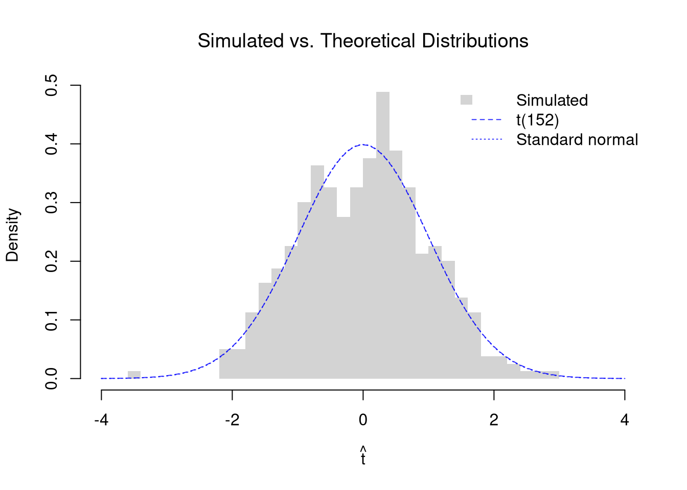
We can also simulate under the null with normally distributed data, where the \(t\)-distribution result applies more directly. Here the two groups have the same mean but different variances.

# Simulate the t-statistic under the null (both groups same mean)
n_sim <- 399
t_sim_norm <- vector(length = n_sim)
for (b in seq(n_sim)) {
    y1_sim_b <- rnorm(n1, 0, 2)
    y2_sim_b <- rnorm(n2, 0, 1)
    t_sim_norm[b] <- t.test(y1_sim_b, y2_sim_b, var.equal = FALSE)$statistic
}

# Welch-Satterthwaite degrees of freedom
# (use population variances as approximation)
v1_norm <- 2^2 / n1
v2_norm <- 1^2 / n2
df_ws_norm <- (v1_norm + v2_norm)^2 / (v1_norm^2 / (n1 - 1) + v2_norm^2 / (n2 - 1))

# Overlay: simulated histogram vs. theoretical t-distribution
t_range <- range(c(t_sim_norm, -4, 4))
hist(t_sim_norm, breaks = 30, freq = FALSE, border = NA,
    xlim = t_range,
    xlab = expression(hat(t)),
    main = NA)
title('Simulated vs. Theoretical Distributions', font.main = 1)
t_grid <- seq(t_range[1], t_range[2], length = 200)
lines(t_grid, dt(t_grid, df = df_ws_norm), col = rgb(0, 0, 1, .8), lty = 2)
lines(t_grid, dnorm(t_grid), col = rgb(0, 0, 1, .8), lty = 3) # standard normal, for z
legend('topright', legend = c('Simulated', paste0('t(', round(df_ws_norm), ')'), 'Standard normal'),
    fill = c(grey(.83), NA, NA), border = NA, # grey(.83) matches the default histogram fill
    lwd = c(NA, 1, 1), lty = c(NA, 2, 3), col = c(NA, rgb(0, 0, 1, .8), rgb(0, 0, 1, .8)), bty = 'n')

Regression Slope

The same ideas apply to regression coefficients. Recall that the OLS slope \(\hat{b}_{1} = \hat{c}_{XY}/\hat{v}_{X}\) is a statistic computed from the data. In the Simple Regression chapter, we estimated variability using data-driven methods (jackknife and bootstrap). Under standard assumptions, we can instead derive the sampling distribution analytically: the \(t\)-statistic \[ \hat{t} = \frac{\hat{b}_{1}}{\hat{\text{SE}}(B_{1})} \] follows a \(t\)-distribution with \(n-2\) degrees of freedom, where \(\hat{\text{SE}}(B_{1})\) is the classical estimated standard error of the slope. This allows us to test \(H_{0}: \beta_{1} = 0\) using math alone. In large samples, the OLS slope is approximately normal even when the errors are not, so the same ratio can also be read as a \(z\)-statistic, \(\hat{z}=\hat{b}_{1}/\hat{\text{SE}}(B_{1})\), and compared to the standard normal.

## MAIN EXAMPLE
# Wages1 data (same as Simple Regression chapter)
data(Wages1, package='Ecdat')
xy_hat <- Wages1[, c('school', 'wage')]
colnames(xy_hat) <- c('x_hat', 'y_hat') # x_hat=years of schooling, y_hat=hourly wage
reg <- lm(y_hat ~ x_hat, data = xy_hat)

# The summary reports theoretical t-statistics and p-values
summary(reg)$coefficients
##               Estimate Std. Error   t value     Pr(>|t|)
## (Intercept) -0.7225066 0.38739136 -1.865056 6.226247e-02
## x_hat        0.5571617 0.03297502 16.896478 1.734818e-61
# Each extra year of schooling goes with about 0.56 more dollars per hour.
# The t-statistic of about 16.9 makes the test of no slope decisive.

NoteMust Know

Manual verification of the theoretical \(t\)-statistic for the slope:

n <- nrow(xy_hat)
b1_hat <- coef(reg)[2]
e_hat <- resid(reg)
s_adj_hat <- sqrt(sum(e_hat^2) / (n - 2)) # root of the adjusted MSE; summary() prints it as the residual standard error
s_b1 <- s_adj_hat / sqrt(sum((xy_hat[, 'x_hat'] - mean(xy_hat[, 'x_hat']))^2)) # SE of slope
t_stat <- b1_hat / s_b1

# Compare with summary output
c(manual = t_stat, summary = summary(reg)$coefficients[2, 3])
## manual.x_hat      summary 
##     16.89648     16.89648

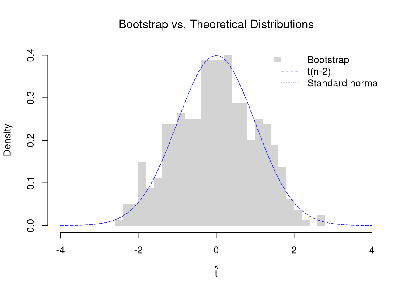
We can compare the bootstrap sampling distribution of \(\hat{t}\) (histogram) with the theoretical \(t_{n-2}\) distribution (dashed curve) and the standard normal (dotted curve). Each bootstrap \(\hat{t}\) is centered at the original slope estimate, which plays the role of the true slope in the bootstrap world. So the histogram approximates the distribution of \(\hat{t}\) when the null is true. They should be similar, but are not identical because the theoretical result assumes normally distributed errors.

# Bootstrap distribution of the t-statistic
n <- nrow(xy_hat)
b1_hat <- coef(reg)[2]
n_boot <- 399
boot_t <- vector(length = n_boot)
for (b in seq(n_boot)) {
    b_id <- sample(nrow(xy_hat), replace = TRUE)
    xy_boot <- xy_hat[b_id, ]
    reg_b <- lm(y_hat ~ x_hat, data = xy_boot)
    # Center at the original estimate and use the theoretical SE from summary
    coef_b <- summary(reg_b)$coefficients[2, ]
    boot_t[b] <- (coef_b[1] - b1_hat) / coef_b[2]
}

# Overlay: bootstrap histogram vs. theoretical t-distribution
t_range <- range(c(boot_t, -4, 4))
hist(boot_t, breaks = 30, freq = FALSE, border = NA,
    xlim = t_range,
    xlab = expression(hat(t)),
    main = NA)
title('Bootstrap vs. Theoretical Distributions', font.main = 1)
# Theoretical t(n-2) density, and the standard normal for z
t_grid <- seq(t_range[1], t_range[2], length = 200)
lines(t_grid, dt(t_grid, df = n - 2), col = rgb(0, 0, 1, .8), lty = 2)
lines(t_grid, dnorm(t_grid), col = rgb(0, 0, 1, .8), lty = 3)
legend('topright', legend = c('Bootstrap', 't(n-2)', 'Standard normal'),
    fill = c(grey(.83), NA, NA), border = NA, # grey(.83) matches the default histogram fill
    lwd = c(NA, 1, 1), lty = c(NA, 2, 3), col = c(NA, rgb(0, 0, 1, .8), rgb(0, 0, 1, .8)), bty = 'n')

# The histogram roughly follows the two curves, which lie on top of each other.
# Wage errors are right-skewed, but with 3294 workers the slope is near normal.
# The observed t of about 16.9 is far off this axis.

We can compute the \(p\)-value for \(H_{0}: \beta_{1} = 0\) three ways: from the theoretical \(t\)-distribution, from the standard normal, and from the bootstrap distribution. All three ask how extreme the observed \(\hat{t}\) is under the null.

t_obs <- summary(reg)$coefficients[2, 3]

# Theoretical p-value: Prob(|t| >= |t_obs|) under t(n-2)
p_theory <- 2 * pt(-abs(t_obs), df = n - 2)

# Normal p-value: the same ratio read as a z-statistic
p_normal <- 2 * pnorm(-abs(t_obs))

# Bootstrap p-value: fraction of bootstrap |t|'s >= |t_obs|
p_boot <- mean(abs(boot_t) >= abs(t_obs))

c(t=p_theory, z=p_normal, bootstrap=p_boot)
##            t            z    bootstrap 
## 1.734818e-61 4.775986e-64 0.000000e+00
# All three are essentially zero, because the observed t is about 16.9.
# The t and z values differ by a large ratio only this far into the tails.
# No bootstrap t came close, so the bootstrap p-value prints as exactly 0.
# With 399 resamples, that only says the p-value is probably below about 3/399, or 0.008.

The \(t_{n-2}\) distribution gets closer to the standard normal as \(n\) grows, so the \(t\) and \(z\) \(p\)-values differ less in larger samples.

TipTest Yourself

Repeat the slope test for the \(50\) states in USArrests, regressing murder arrests on the urban population share. How far apart are the \(t\) and \(z\) \(p\)-values with this many observations?

# Murder arrests per 100K and urban population share, 50 US states, 1973
xy2_hat <- USArrests[, c('UrbanPop', 'Murder')]
colnames(xy2_hat) <- c('x_hat', 'y_hat') # x_hat=urban population share, y_hat=murder arrests per 100K
reg2 <- lm(y_hat ~ x_hat, data = xy2_hat)

# The summary reports theoretical t-statistics and p-values
summary(reg2)$coefficients
##               Estimate Std. Error   t value   Pr(>|t|)
## (Intercept) 6.41594246 2.90669257 2.2073000 0.03210725
## x_hat       0.02093466 0.04332647 0.4831841 0.63116178
# The slope is about 0.02, only about half of its standard error.

# Bootstrap distribution of the t-statistic
n2 <- nrow(xy2_hat)
slope2_hat <- coef(reg2)[2]
n_boot <- 399
boot_t2 <- vector(length = n_boot)
for (b in seq(n_boot)) {
    b_id <- sample(nrow(xy2_hat), replace = TRUE)
    xy2_boot <- xy2_hat[b_id, ]
    reg2_b <- lm(y_hat ~ x_hat, data = xy2_boot)
    # Center at the original estimate and use the theoretical SE from summary
    coef2_b <- summary(reg2_b)$coefficients[2, ]
    boot_t2[b] <- (coef2_b[1] - slope2_hat) / coef2_b[2]
}

# Overlay: bootstrap histogram vs. theoretical t-distribution
t_range2 <- range(c(boot_t2, -4, 4))
hist(boot_t2, breaks = 30, freq = FALSE, border = NA,
    xlim = t_range2,
    xlab = expression(hat(t)),
    main = NA)
title('Bootstrap vs. Theoretical Distributions', font.main = 1)
# Theoretical t(n-2) density, and the standard normal for z
t_grid2 <- seq(t_range2[1], t_range2[2], length = 200)
lines(t_grid2, dt(t_grid2, df = n2 - 2), col = rgb(0, 0, 1, .8), lty = 2)
lines(t_grid2, dnorm(t_grid2), col = rgb(0, 0, 1, .8), lty = 3)
legend('topright', legend = c('Bootstrap', 't(n-2)', 'Standard normal'),
    fill = c(grey(.83), NA, NA), border = NA, # grey(.83) matches the default histogram fill
    lwd = c(NA, 1, 1), lty = c(NA, 2, 3), col = c(NA, rgb(0, 0, 1, .8), rgb(0, 0, 1, .8)), bty = 'n')

t_obs2 <- summary(reg2)$coefficients[2, 3]

# Theoretical p-value: Prob(|t| >= |t_obs2|) under t(n-2)
p_theory2 <- 2 * pt(-abs(t_obs2), df = n2 - 2)

# Normal p-value: the same ratio read as a z-statistic
p_normal2 <- 2 * pnorm(-abs(t_obs2))

# Bootstrap p-value: fraction of bootstrap |t|'s >= |t_obs2|
p_boot2 <- mean(abs(boot_t2) >= abs(t_obs2))

c(t=p_theory2, z=p_normal2, bootstrap=p_boot2)
##         t         z bootstrap 
## 0.6311618 0.6289650 0.6616541
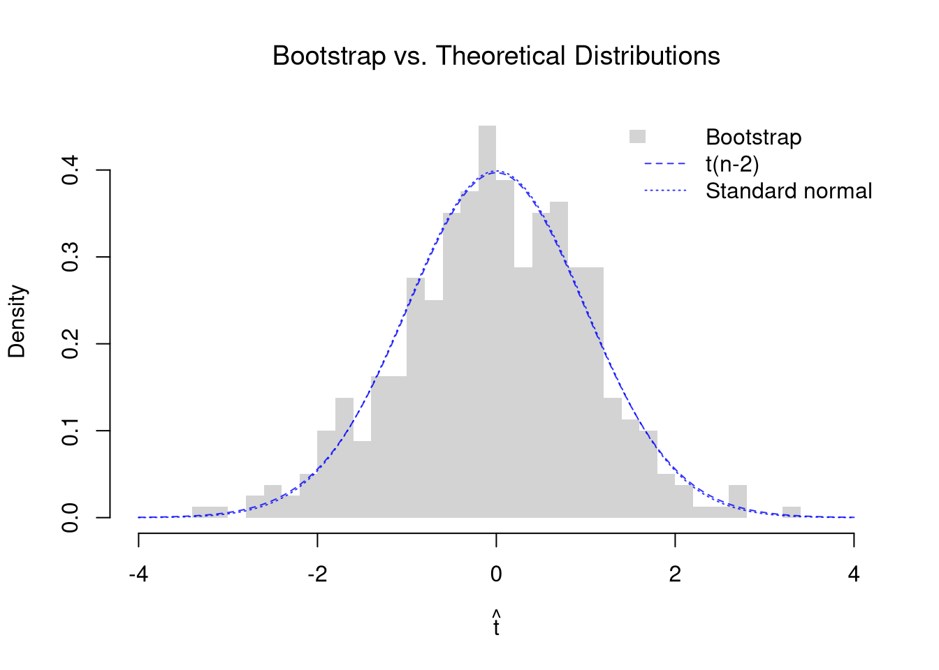
# With 50 states, t(48) is already close to the standard normal.
# So the t and z p-values agree to two decimal places.

The same ratio can test other hypothesized values \(\beta_{1}\) of the population slope. To impose the null, recenter the numerator around the hypothetical value: \(\hat{t} = \frac{\hat{b}_{1} - \beta_{1}}{\hat{\text{SE}}(B_{1})}\), as we did for the mean in \(t\)-values. Under the same assumptions as above, this \(\hat{t}\) also follows a \(t\)-distribution with \(n-2\) degrees of freedom when the null is true.

# Recenter at a hypothesized slope of 0.5 dollars per year of schooling
beta1_null <- 0.5
se_hat <- summary(reg)$coefficients[2, 2]
t_null <- unname(b1_hat - beta1_null) / se_hat
t_null
## [1] 1.733485

# The same three p-values, now for this null
c(t=2 * pt(-abs(t_null), df=n - 2),
    z=2 * pnorm(-abs(t_null)),
    bootstrap=mean(abs(boot_t) >= abs(t_null)))
##          t          z  bootstrap 
## 0.08310318 0.08300955 0.09022556
# With 3294 workers, the t and z p-values match to three decimal places.
# The bootstrap p-value is near them, and it moves with the random draws.

TipTest Yourself

Redo the bootstrap \(p\)-value with the jackknife standard error in place of the classical one. Recompute the jackknife standard error inside each bootstrap resample. Refitting the model \(n\) times per resample can be slow, so the code below gets all the leave-one-out slopes from one fit with lm.influence().

# Jackknife SE of the slope and the observed t
jack_coefs <- rep(NA, n)
for (i in seq_along(jack_coefs)) {
    xy_i <- xy_hat[-i, ]
    jack_coefs[i] <- coef(lm(y_hat ~ x_hat, data = xy_i))[2]
}
jack_se <- sqrt((n - 1)/n * sum((jack_coefs - mean(jack_coefs))^2))
t_jack <- b1_hat / jack_se

# lm.influence() reports how much each coefficient moves when row i is dropped.
# So it gives the same slopes as the loop above, without refitting.
all.equal(jack_coefs, unname(b1_hat - lm.influence(reg)$coefficients[, 2]))
## [1] TRUE

# Bootstrap t, with a jackknife SE for each resample
# Refitting here would mean about 1.3 million fits (3294 times 399)
boot_t_jack <- rep(NA, n_boot)
for (b in seq(n_boot)) {
    b_id <- sample(n, replace = TRUE)
    xy_boot <- xy_hat[b_id, ]
    reg_b <- lm(y_hat ~ x_hat, data = xy_boot)
    slope_b <- coef(reg_b)[2]
    jack_coefs_b <- slope_b - lm.influence(reg_b)$coefficients[, 2]
    jack_se_b <- sqrt((n - 1)/n * sum((jack_coefs_b - mean(jack_coefs_b))^2))
    # Center at the original estimate, as above
    boot_t_jack[b] <- (slope_b - b1_hat) / jack_se_b
}

# Classical t p-value next to the bootstrap p-value with jackknife SEs
c(classical=p_theory, jackknife_boot=mean(abs(boot_t_jack) >= abs(t_jack)))
##      classical jackknife_boot 
##   1.734818e-61   0.000000e+00
# Both are essentially zero, so the test of no slope is decisive either way.

# The same comparison at the hypothesized slope of 0.5
t_jack_null <- unname(b1_hat - beta1_null) / jack_se
c(classical=2 * pt(-abs(t_null), df=n - 2),
    jackknife_boot=mean(abs(boot_t_jack) >= abs(t_jack_null)))
##      classical jackknife_boot 
##     0.08310318     0.08270677

# The two standard errors are close, so the two tests tend to agree
c(classical=se_hat, jackknife=jack_se)
##  classical  jackknife 
## 0.03297502 0.03355489

TipTest Yourself

Checking with a Known Population

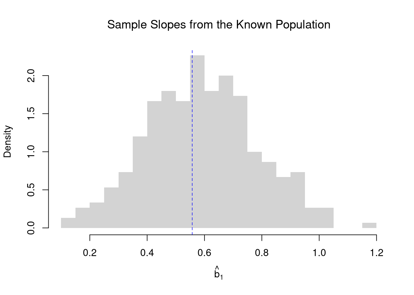
A \(95\%\) confidence interval should contain the population slope in about \(95\%\) of samples. With real data, we never see the population slope, so we cannot check whether our intervals work. As in Sampling, pretend the \(3294\) workers in Wages1 are the whole population, so we know the population slope of wages on schooling. We then draw many samples of \(n=100\) workers, fit a regression on each, and see how the sample slopes scatter around the population slope.

# Pretend these 3294 workers are the whole population
data(Wages1, package='Ecdat')
population_xy <- Wages1[, c('school', 'wage')]
colnames(population_xy) <- c('x', 'y') # x=years of schooling, y=hourly wage
population_slope <- coef(lm(y ~ x, data=population_xy))[2]
population_slope
##         x 
## 0.5571617

# Draw many samples and fit a regression on each
n <- 100
slopes_sim <- rep(NA, 300)
for(s in seq_along(slopes_sim)){
    s_id <- sample(nrow(population_xy), n, replace=FALSE)
    xy_sim <- population_xy[s_id, ]
    colnames(xy_sim) <- c('x_hat', 'y_hat')
    reg_s <- lm(y_hat ~ x_hat, data=xy_sim)
    slopes_sim[s] <- coef(reg_s)[2]
}

# Sampling distribution of the slope
hist(slopes_sim, breaks=25,
    main=NA, border=NA, freq=FALSE,
    xlab=expression(hat(b)[1]))
title('Sample Slopes from the Known Population', font.main=1)
abline(v=population_slope, col=rgb(0, 0, 1, .8), lty=2)

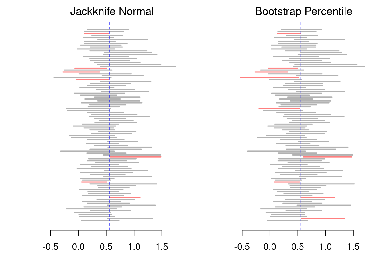
We check the coverage of both intervals from Simple Regression: the jackknife Normal interval and the bootstrap percentile interval. Inside the resampling loops, we compute each slope as \(\hat{c}_{XY}/\hat{v}_{X}\), which gives the same number as lm but runs faster.

# Jackknife Normal CI and bootstrap percentile CI for each sample
n_samples <- 300
jack_cis <- matrix(NA, nrow=n_samples, ncol=2)
boot_cis <- matrix(NA, nrow=n_samples, ncol=2)
for(s in seq(n_samples)){
    s_id <- sample(nrow(population_xy), n, replace=FALSE)
    x_sim <- population_xy[s_id, 'x']
    y_sim <- population_xy[s_id, 'y']
    slope_s <- cov(x_sim, y_sim)/var(x_sim)
    # Jackknife SE and Normal CI
    jack_coefs_s <- rep(NA, n)
    for(i in seq_along(jack_coefs_s)){
        x_sim_i <- x_sim[-i]
        y_sim_i <- y_sim[-i]
        jack_coefs_s[i] <- cov(x_sim_i, y_sim_i)/var(x_sim_i)
    }
    jack_se_s <- sqrt((n - 1)/n * sum((jack_coefs_s - mean(jack_coefs_s))^2))
    jack_cis[s, ] <- qnorm(c(.025, .975), slope_s, jack_se_s)
    # Bootstrap percentile CI
    boot_coefs_s <- rep(NA, 399)
    for(b in seq_along(boot_coefs_s)){
        b_id <- sample(n, replace=TRUE)
        x_sim_boot <- x_sim[b_id]
        y_sim_boot <- y_sim[b_id]
        boot_coefs_s[b] <- cov(x_sim_boot, y_sim_boot)/var(x_sim_boot)
    }
    boot_cis[s, ] <- quantile(boot_coefs_s, probs=c(.025, .975))
}

# Percent of intervals that contain the population slope
jack_covered <- population_slope >= jack_cis[, 1] & population_slope <= jack_cis[, 2]
boot_covered <- population_slope >= boot_cis[, 1] & population_slope <= boot_cis[, 2]
c(jackknife_normal=mean(jack_covered), bootstrap_percentile=mean(boot_covered))*100
##     jackknife_normal bootstrap_percentile 
##                   94                   91
# Both percents are typically a little below 95%, the bootstrap more so.
# Wages are right-skewed, so neither interval is exact with n=100.

# Plot the first 100 intervals from each method (Red = Missed)
cis_list <- list('Jackknife Normal'=jack_cis[1:100, ], 'Bootstrap Percentile'=boot_cis[1:100, ])
ci_xlim <- range(jack_cis[1:100, ], boot_cis[1:100, ])
par(mfrow=c(1, 2), mar=c(4, 4, 2, 1))
for(method in names(cis_list)){
    cis <- cis_list[[method]]
    covered <- population_slope >= cis[, 1] & population_slope <= cis[, 2]
    plot.new()
    plot.window(xlim=ci_xlim, ylim=c(0, 100))
    segments(cis[, 1], 1:100, cis[, 2], 1:100, lwd=2,
        col=ifelse(covered, rgb(0, 0, 0, .3), rgb(1, 0, 0, .5)))
    abline(v=population_slope, col=rgb(0, 0, 1, .8), lty=2)
    axis(1)
    title(method, font.main=1)
}

Some of any gap between the printed percents and \(95\%\) is simulation noise from using a limited number of samples. The rest is because neither interval is exact: with skewed data, the sampling distribution of the slope is not exactly Normal, and the bootstrap distribution only approximates it.

NoteMust Know

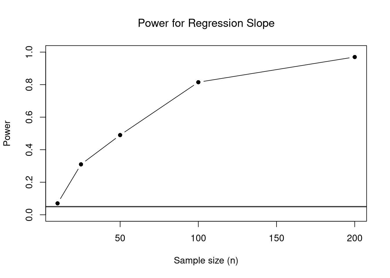
We can also compute the Type I Error rate and power of the theoretical test from a simulated data generating process, where we set the true slope ourselves. The process below is calibrated to the regression above, with normally distributed \(X_{i}\) and errors.

alpha <- 0.05

# DGP calibrated to the regression of wages on schooling
beta0 <- coef(reg)[1]
beta1_true <- coef(reg)[2]
s_adj_hat <- summary(reg)$sigma
m_x_hat <- mean(xy_hat[, 'x_hat'])
s_adj_x_hat <- sd(xy_hat[, 'x_hat'])

# Function: simulate data, return theoretical p-value for slope
sim_pval <- function(n, beta1) {
    x_sim <- rnorm(n, mean = m_x_hat, sd = s_adj_x_hat)
    y_sim <- beta0 + beta1 * x_sim + rnorm(n, 0, s_adj_hat)
    summary(lm(y_sim ~ x_sim))$coefficients[2, 4]
}

sim_reps_dgp <- 200

# Type I Error rate: true slope = 0
pvals_null <- replicate(sim_reps_dgp, sim_pval(n = 50, beta1 = 0))
type1_rate_dgp <- mean(pvals_null < alpha)
type1_rate_dgp  # should be close to alpha
## [1] 0.06

# Power: true slope = beta1_true
pvals_alt <- replicate(sim_reps_dgp, sim_pval(n = 50, beta1 = beta1_true))
power_dgp <- mean(pvals_alt < alpha)
power_dgp
## [1] 0.595
# With 50 workers, the test detects this slope a little over half of the time.

# Power increases with sample size
n_grid_dgp <- c(10, 25, 50, 100, 200)
power_by_n_dgp <- sapply(n_grid_dgp, function(ni) {
    pvals <- replicate(sim_reps_dgp, sim_pval(ni, beta1 = beta1_true))
    mean(pvals < alpha)
})

plot(n_grid_dgp, power_by_n_dgp, type = 'b', pch = 16,
    xlab = 'Sample size (n)', ylab = 'Power',
    ylim = c(0, 1),
    main = NA)
title('Power for Regression Slope', font.main = 1)
abline(h = alpha, col = rgb(0, 0, 0, .8), lwd = 2)

# Power climbs from about 0.1 with 10 workers to nearly 1 with 200.
# With all 3294 workers, power would be essentially 1.

Differences in Medians

If we want to test for the differences in medians across groups with independent observations, we can also use notches in the boxplot, as in Multiple Groups. R’s default notches (notch=TRUE) come from a normal-theory approximation. Let each group \(g\) have median \(\tilde{m}_{Y}(g)\), interquartile range \(\hat{\text{IQR}}_{Y}(g)\), observations \(n_{g}\). We can compute standard deviation of the median as \(\tilde{S}_{Y}(g)= \frac{1.25 \hat{\text{IQR}}_{Y}(g)}{1.35 \sqrt{n_{g}}}\). As a rough guess, the interval \(\tilde{m}_{Y}(g) \pm 1.7 \tilde{S}_{Y}(g)\) is the historical default and displayed as a notch in the boxplot (McGill et al. 1978).

The same standard errors give a \(z\)-statistic for the difference in medians, \[\hat{z} = \frac{\tilde{m}_{Y}(1)-\tilde{m}_{Y}(2)}{\sqrt{\tilde{S}_{Y}(1)^2+\tilde{S}_{Y}(2)^2}}.\] Unlike \(\hat{t}\) for means, this ratio has no \(t\)-distribution result, even when the data are normal, so we compare it to the standard normal, which is accurate only in large samples. The standard error of a median depends on how dense the data are near the median, and \(\tilde{S}_{Y}(g)\) fills that in by assuming normality. Specifically, \(\hat{\text{IQR}}_{Y}(g)/1.35\) estimates the standard deviation of normal data, and \(1.25\approx\sqrt{\pi/2}\) is how much more variable a sample median is than a sample mean when the data are normal. Two notches do not overlap when \(|\tilde{m}_{Y}(1)-\tilde{m}_{Y}(2)| > 1.7[\tilde{S}_{Y}(1)+\tilde{S}_{Y}(2)]\). With equal standard errors, that is the same as \(|\hat{z}| > 1.7\sqrt{2} \approx 2.4\), a stricter cutoff than \(1.96\), which is why overlapping notches do not show that the medians are equal.

NoteMust Know

Suppose two groups of \(n_{1}=n_{2}=100\) workers have median wages \(\tilde{m}_{Y}(1)=17\) and \(\tilde{m}_{Y}(2)=15\), and both have an interquartile range of \(7\). Each standard error is \(\tilde{S}_{Y}(g)=1.25\times 7/(1.35\times 10)\approx 0.648\), so \[\hat{z} = \frac{17-15}{\sqrt{0.648^2+0.648^2}} \approx \frac{2}{0.917} \approx 2.18,\] with a \(p\)-value of about \(0.029\). Each notch extends \(1.7\times 0.648\approx 1.10\) from its median, so the notches \([15.90, 18.10]\) and \([13.90, 16.10]\) overlap. So the \(z\)-statistic rejects at the \(5\%\) level even though the notches overlap.

## MAIN EXAMPLE
# Two groups of 100 workers with the same interquartile range
n0 <- 100
med01_hat <- 17
med02_hat <- 15
iqr0_hat <- 7

# Normal-theory standard error of each median
se0_hat <- 1.25 * iqr0_hat / (1.35 * sqrt(n0))

# z-statistic and its two-sided p-value
z0_hat <- (med01_hat - med02_hat) / sqrt(se0_hat^2 + se0_hat^2)
c(se=se0_hat, z=z0_hat, p_value=2 * pnorm(-abs(z0_hat)))
##         se          z    p_value 
## 0.64814815 2.18192950 0.02911474

# Notches: each median plus or minus 1.7 standard errors
rbind(group1=med01_hat + c(-1.7, 1.7) * se0_hat,
    group2=med02_hat + c(-1.7, 1.7) * se0_hat)
##            [,1]     [,2]
## group1 15.89815 18.10185
## group2 13.89815 16.10185

TipTest Yourself

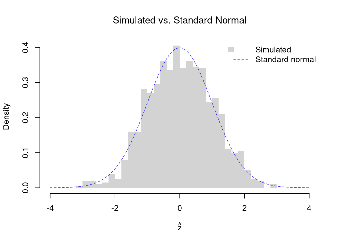
Check how well the standard normal describes \(\hat{z}\) when the null is true. As in the simulation for means above, draw both groups from the pretend population of Wages1 workers, so the two population medians are equal. With \(50\) workers per group, about \(5\%\) of the samples should have \(|\hat{z}|>1.96\). The standard normal is only a large-sample approximation, so repeat the check with n_g at \(10\).

# Draw both groups from the same pretend population, so the medians are equal
n_g <- 50
n_sim <- 999
z_sim <- rep(NA, n_sim)
for (b in seq(n_sim)) {
    y1_sim_b <- sample(population_wages, n_g)
    y2_sim_b <- sample(population_wages, n_g)
    se1_b <- 1.25 * IQR(y1_sim_b) / (1.35 * sqrt(n_g)) # normal-theory SE of each median
    se2_b <- 1.25 * IQR(y2_sim_b) / (1.35 * sqrt(n_g))
    z_sim[b] <- (median(y1_sim_b) - median(y2_sim_b)) / sqrt(se1_b^2 + se2_b^2)
}

# Share of samples with |z| > 1.96, near 5% if the standard normal fits
mean(abs(z_sim) > 1.96)
## [1] 0.05105105
# Change n_g to 10 and the share rises.

# Overlay: simulated histogram vs. standard normal
z_range <- range(c(z_sim, -4, 4))
hist(z_sim, breaks=30, freq=FALSE, border=NA,
    xlim=z_range, xlab=expression(hat(z)), main=NA)
title('Simulated vs. Standard Normal', font.main=1)
z_grid <- seq(z_range[1], z_range[2], length=200)
lines(z_grid, dnorm(z_grid), col=rgb(0, 0, 1, .8), lty=2)
legend('topright', legend=c('Simulated', 'Standard normal'),
    fill=c(grey(.83), NA), border=NA, # grey(.83) matches the default histogram fill
    lwd=c(NA, 1), lty=c(NA, 2), col=c(NA, rgb(0, 0, 1, .8)), bty='n')

19.2 Bias-Variance Tradeoff

A better fit on the data you have is not automatically better, because a model can hit every point in the sample and still predict new observations poorly.

ImportantKey Definition

Let \(Y^{\mathrm{pred}}(x)\) be a model’s prediction at \(x\) before the sample is drawn, and let \(m_{Y}(x)=\mathbb{E}[Y_{i}\mid X_{i}=x]\) be the conditional expectation it estimates. The mean squared error of the prediction decomposes into two pieces: \[\mathbb{E}\left[\left(Y^{\mathrm{pred}}(x)-m_{Y}(x)\right)^2\right] = \left(\mathbb{E}\left[Y^{\mathrm{pred}}(x)\right]-m_{Y}(x)\right)^2 + \mathbb{V}\left[Y^{\mathrm{pred}}(x)\right].\] Squared bias, the first piece, is how far the average prediction sits from the truth. Variance, the second piece, is how much the predictions wobble around their own average. The bias-variance tradeoff is that cutting one piece usually raises the other.

The bias-variance tradeoff is useful for thinking about why a tuning parameter matters and how to set it. For local regressions, the bandwidth \(h\) (for LOESS, the span) controls the tradeoff. A large \(h\) lowers variance but raises bias, and a small \(h\) does the opposite. A loess fit narrow enough to interpolate every point has \(\hat{\text{MSE}}=0\) on the fit data, as defined in Model Fit, but generalizes poorly because it has just copied the noise.

• Wide window (large span, large \(h\)): each local fit uses many observations, so the fitted curve barely changes from sample to sample (low variance). But a nearly flat fit over a wide region cannot follow a relationship that bends, so it is systematically off (high bias).
• Narrow window (small span, small \(h\)): each local fit uses few observations, so the fitted curve chases noise and swings from sample to sample (high variance). But a narrow window can track curvature closely (low bias).

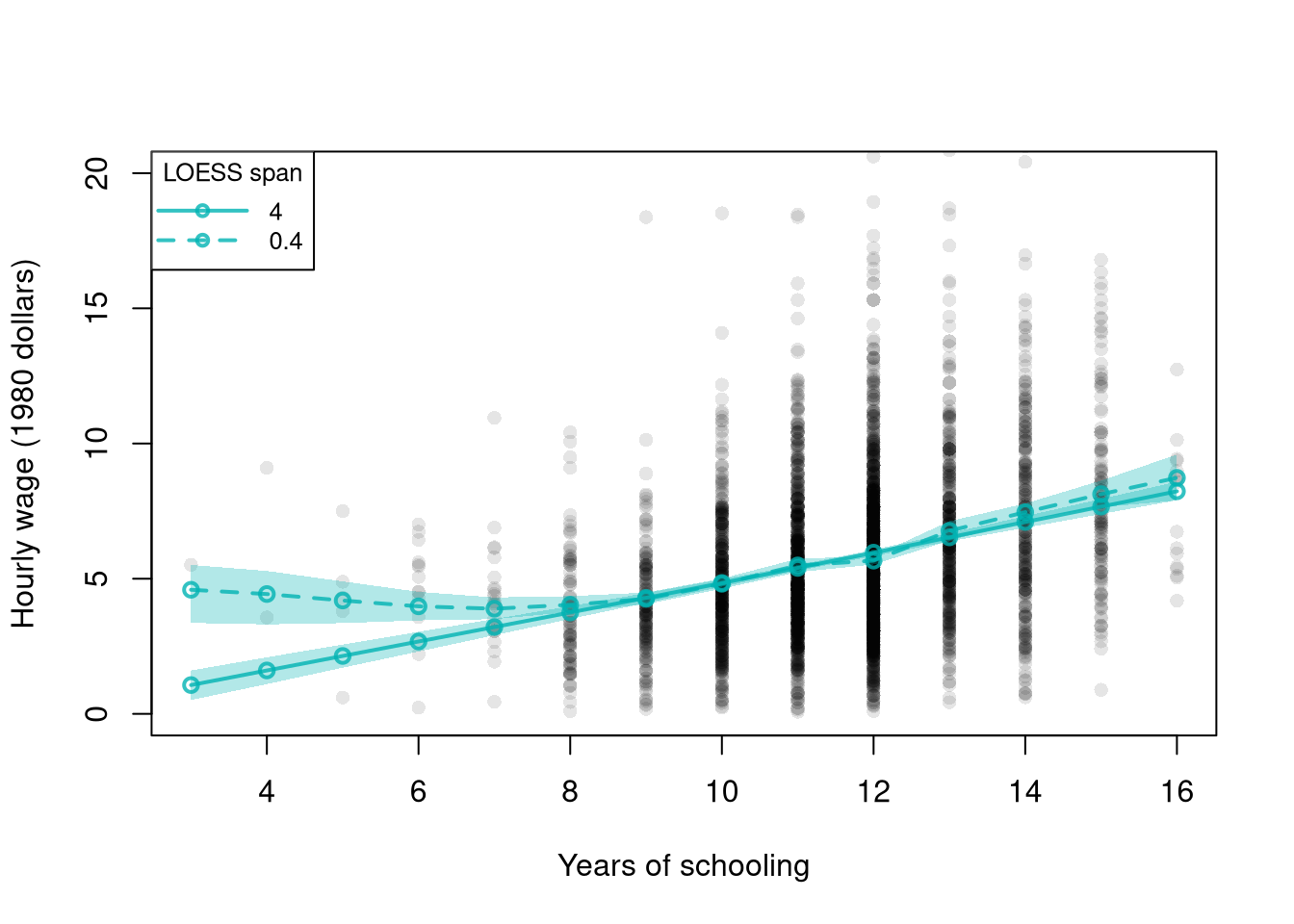
This section fits local linear LOESS (degree=1), which is more stable than the default local quadratic in small samples.

# Lab data from above: wages and schooling for 3294 workers
# Schooling takes only a few distinct values, so all fits here are local linear

# Two-span local linear loess with bootstrap confidence bands on one scatterplot
pred_design <- data.frame(x_hat=sort(unique(xy_hat[, 'x_hat'])))
# Schooling is an integer, and about a third of workers have exactly 12 years.
# Spans below about 0.4 leave no other schooling level near 12.
# So loess() breaks down there.
spans <- c(4.0, 0.4)
n_boot <- 399
span_lty <- c(1, 2) # both spans are LOESS, so they share a color and differ by line type

# The axis stops just past 20 dollars, so the 16 largest wages are not drawn
plot(y_hat ~ x_hat, data=xy_hat, pch=16, col=grey(0, .1),
    ylim=c(0, 20),
    main=NA, xlab='Years of schooling', ylab='Hourly wage (1980 dollars)')

for (s in seq_along(spans)) {
    sp <- spans[s]
    reg_s <- loess(y_hat ~ x_hat, data=xy_hat, span=sp, degree=1)
    boot_preds <- matrix(NA, nrow=nrow(pred_design), ncol=n_boot)
    for (b in 1:n_boot) {
        xy_boot <- xy_hat[sample(nrow(xy_hat), replace=TRUE), ]
        reg_s_b <- loess(y_hat ~ x_hat, data=xy_boot, span=sp, degree=1)
        boot_preds[, b] <- predict(reg_s_b, newdata=pred_design)
    }
    boot_cb <- apply(boot_preds, 1, quantile,
        probs=c(.025, .975), na.rm=TRUE)

    polygon(c(pred_design[, 'x_hat'], rev(pred_design[, 'x_hat'])),
        c(boot_cb[1, ], rev(boot_cb[2, ])),
        col=rgb(0, .7, .7, .3), border=NA)
    lines(pred_design[, 'x_hat'], predict(reg_s, newdata=pred_design),
        col=rgb(0, .7, .7, .8), lwd=2, lty=span_lty[s], type='o')
}

legend('topleft', title='LOESS span',
    legend=paste0(spans),
    col=rgb(0, .7, .7, .8), lty=span_lty, lwd=2, pch=1, cex=.8,
    seg.len=4) # long enough that the circle does not hide the dashes

# With span 4.0 the curve is nearly a straight line and very stable.
# With span 0.4 the curve tracks more local variation, and its band fans wider.

A wider span gives a more stable curve and a tighter bootstrap band, while a narrower span tracks more local variation. Following local detail raises the variance.

With local linear fits, a very wide span gives every observation nearly the same weight, so the fit approaches the simple linear regression as \(h \to \infty\). A wide window and a narrow window can therefore also be read as a linear model and a flexible LOESS fit.

The bootstrap bands show variance, but not bias, because we never see the true curve in one sample. As in Sampling, pretend the data are the whole population, so the true curve is known. The population curve is the mean outcome at each value of the explanatory variable, over the whole population. We evaluate it only at values with many observations. The rest of this section compares the linear model, which acts as the widest possible window, with LOESS at span \(0.6\).

## MAIN EXAMPLE
# Wages1 defined above
# Pretend these 3294 workers are the whole population
population_xy <- Wages1[, c('school', 'wage')]
colnames(population_xy) <- c('x', 'y') # x=years of schooling, y=hourly wage

# Population curve: mean wage at each schooling level
population_curve <- tapply(population_xy[, 'y'], population_xy[, 'x'], mean)

# Evaluate at schooling levels with many workers (8 to 15 years)
# Rare levels are often missing from a sample, and loess does not extrapolate
x_levels <- 8:15
population_levels <- population_curve[as.character(x_levels)]

# Draw a simple random sample of n workers from the population
draw_xy <- function(n=300){
    s_id <- sample(nrow(population_xy), n, replace=FALSE)
    xy_sim <- population_xy[s_id, ]
    colnames(xy_sim) <- c('x_hat', 'y_hat')
    return(xy_sim)
}

# Span for all local linear fits in the main text
span_wage <- 0.6

Bias

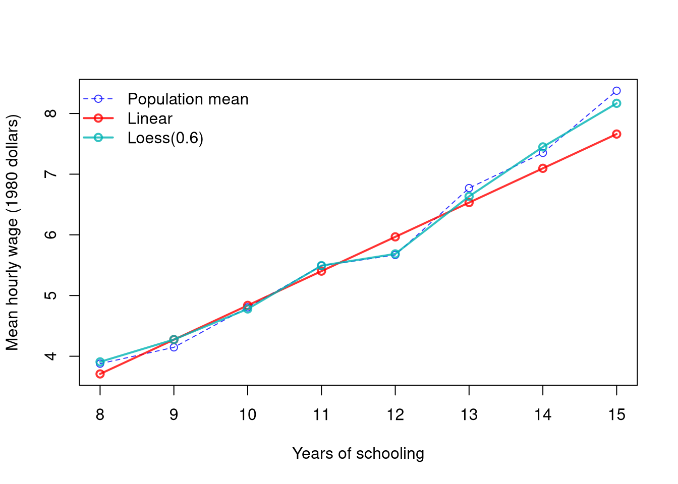
The plot below shows the average prediction across many samples against the population mean at each value. LOESS can track the population curve closely.¹ A linear model can do so only where the population curve is straight.

## MAIN EXAMPLE
## Shared settings used by Bias, Variance, and the Decomposition
n_rep <- 300
n_seq <- c(50, 100, 200, 400, 800)
n_bias <- 200
x_target <- 12 # high school graduates

## Predictions at x_target: one row per sample, one column per sample size
target_lm_sim <- matrix(NA, nrow=n_rep, ncol=length(n_seq))
target_lo_sim <- matrix(NA, nrow=n_rep, ncol=length(n_seq))

## Predictions at every schooling level when n == n_bias
curves_lm_sim <- matrix(NA, nrow=length(x_levels), ncol=n_rep)
curves_lo_sim <- matrix(NA, nrow=length(x_levels), ncol=n_rep)

## One sweep over sample sizes
for (ni in seq_along(n_seq)) {
    n <- n_seq[ni]
    for (r in 1:n_rep) {
        xy_sim <- draw_xy(n)
        reg_lm <- lm(y_hat ~ x_hat, data=xy_sim)
        reg_lo <- loess(y_hat ~ x_hat, data=xy_sim, span=span_wage, degree=1)
        y_pred_lm <- predict(reg_lm, newdata=data.frame(x_hat=x_levels))
        y_pred_lo <- predict(reg_lo, newdata=data.frame(x_hat=x_levels))
        target_lm_sim[r, ni] <- y_pred_lm[x_levels == x_target]
        target_lo_sim[r, ni] <- y_pred_lo[x_levels == x_target]
        if (n == n_bias) {
            curves_lm_sim[, r] <- y_pred_lm
            curves_lo_sim[, r] <- y_pred_lo
        }
    }
}

# Average predictions across the samples of 200 workers
m_lm_hat <- rowMeans(curves_lm_sim, na.rm=TRUE)
m_lo_hat <- rowMeans(curves_lo_sim, na.rm=TRUE)

y_rng <- range(c(population_levels, m_lm_hat, m_lo_hat), na.rm=TRUE)
plot(x_levels, population_levels, type='o', lwd=1, lty=2,
    col=rgb(0, 0, 1, .8), ylim=y_rng,
    xlab='Years of schooling', ylab='Mean hourly wage (1980 dollars)', main=NA)
lines(x_levels, m_lm_hat, type='o', lwd=2, col=rgb(1, 0, 0, .8))
lines(x_levels, m_lo_hat, type='o', lwd=2, col=rgb(0, .7, .7, .8))
legend('topleft', lty=c(2, 1, 1), lwd=c(1, 2, 2), pch=1, bty='n',
    col=c(rgb(0, 0, 1, .8), rgb(1, 0, 0, .8), rgb(0, .7, .7, .8)),
    legend=c('Population mean',
        'Linear',
        paste0('Loess(', span_wage, ')')
))

# LOESS tracks the population curve closely.
# The line is too high at 12 years of schooling and too low at 13 to 15 years.

# reg is the line fit to all 3294 workers, the whole pretend population
y_pred_population <- predict(reg, newdata=data.frame(x_hat=x_target))
c(line=unname(y_pred_population),
    population_mean=population_curve[[as.character(x_target)]])
##            line population_mean 
##        5.963434        5.668354
# At 12 years, it predicts about 5.96 against a population mean of about 5.67.

The linear bias does not go away with more data. Even the line fit to the whole population is only the best linear approximation to the conditional expectation, so, as in the \(3\times3\) example of Bivariate Theory, it misses wherever the conditional expectation bends.

Variance

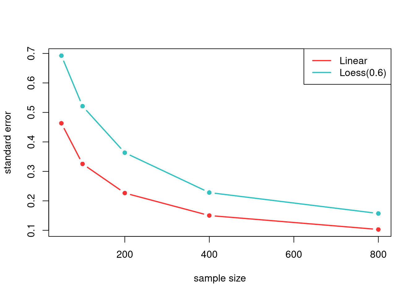
The model estimates also vary from sample to sample. The plot below shows the standard error of each model’s prediction at one target point, computed across the repeated samples. A linear prediction generally varies less than a LOESS prediction, even when it is biased.

Also notice that there are diminishing returns to larger sample sizes. Both predictions vary less from sample to sample as \(n\) grows, making confidence intervals narrower and hypothesis tests more accurate.

# Predicted mean wage at 12 years of schooling, across the repeated samples
se_sim <- rbind(
    apply(target_lm_sim, 2, sd, na.rm=TRUE),
    apply(target_lo_sim, 2, sd, na.rm=TRUE))
cols <- c(rgb(1, 0, 0, .8), rgb(0, .7, .7, .8)) # linear, LOESS
matplot(n_seq, t(se_sim), type='b', pch=16,
    lty=1, lwd=2, col=cols,
    ylab='standard error', xlab='sample size',
    main=NA)
legend('topright',
    lty=1, lwd=2, col=cols,
    legend=c('Linear', paste0('Loess(', span_wage, ')')))

# The linear prediction varies less than LOESS at every sample size here.

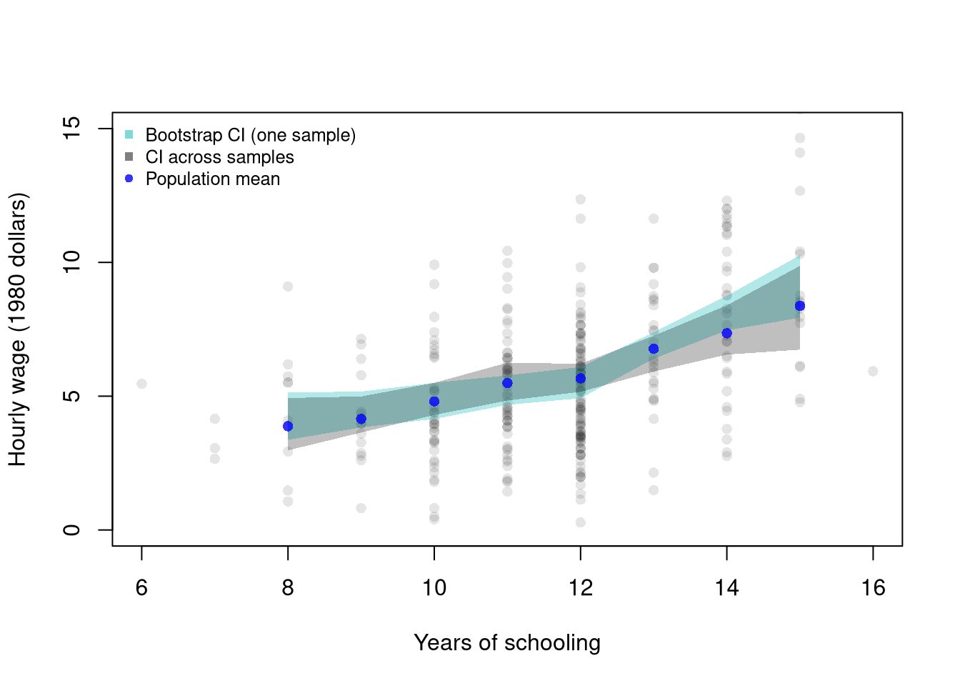
Bootstrap confidence bands are approximations: they estimate how much predicted values vary from sample to sample. The simulation below compares a bootstrap CI constructed from one sample to the true sampling variation observed across many independent samples from the population.

## Data from one sample of 300 workers
xy_sim <- draw_xy(300)
plot(y_hat ~ x_hat, data=xy_sim, pch=16, col=grey(0, .1),
    ylim=c(0, 15), # zoom in on the fitted curves
    main=NA, ylab='Hourly wage (1980 dollars)', xlab='Years of schooling')

## Plot Bootstrap CI for Single Sample
pred_design <- data.frame(x_hat=x_levels)
boot_lo <- matrix(NA, nrow=nrow(pred_design), ncol=399)
for (b in 1:399) {
    xy_boot <- xy_sim[sample(nrow(xy_sim), replace=TRUE), ]
    reg_b <- loess(y_hat ~ x_hat, data=xy_boot, span=span_wage, degree=1)
    boot_lo[, b] <- predict(reg_b, newdata=pred_design)
}
boot_cb <- apply(boot_lo, 1, quantile,
    probs=c(.025, .975), na.rm=TRUE)
polygon(
    c(pred_design[[1]], rev(pred_design[[1]])),
    c(boot_cb[1, ], rev(boot_cb[2, ])),
    col=rgb(0, .7, .7, .3),
    border=NA)

# Construct CI across Multiple Samples from the population
sample_lo <- matrix(NA, nrow=nrow(pred_design), ncol=399)
for (b in 1:399) {
    xy_sim_b <- draw_xy(300) # Entirely new sample
    reg_b <- loess(y_hat ~ x_hat, data=xy_sim_b, span=span_wage, degree=1)
    sample_lo[, b] <- predict(reg_b, newdata=pred_design)
}
ci_lo <- apply(sample_lo, 1, quantile,
    probs=c(.025, .975), na.rm=TRUE)
polygon(
    c(pred_design[[1]], rev(pred_design[[1]])),
    c(ci_lo[1, ], rev(ci_lo[2, ])),
    col=grey(0, alpha=.25),
    border=NA)

# Population curve, in blue as in the Bias plot
points(x_levels, population_levels, pch=16, col=rgb(0, 0, 1, .8))
legend('topleft', bty='n', cex=.8,
    legend=c('Bootstrap CI (one sample)', 'CI across samples', 'Population mean'),
    pch=c(15, 15, 16),
    col=c(rgb(0, .7, .7, .5), grey(0, .5), rgb(0, 0, 1, .8)))

The two bands typically have a similar width, so the bootstrap from one sample gives a reasonable idea of the variation across samples. The bootstrap band is centered on the one sample we happen to have, however, so it can sit a little above or below the population curve.

Bias-Variance Decomposition

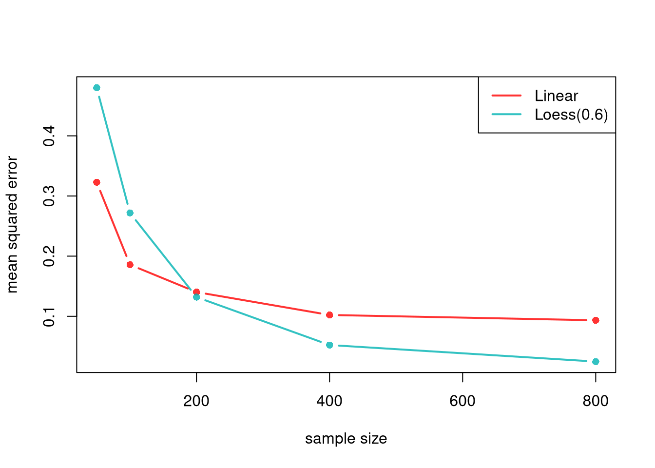
The code below computes the squared bias, the variance, and the mean squared error (MSE) from the definition above, for each model’s prediction at the target point and each sample size.

## MAIN EXAMPLE
# Squared bias, variance, and MSE for each column (sample size)
truth_target <- population_curve[as.character(x_target)] # 12 years of schooling
mse_parts <- function(P, truth){
    bias2 <- (colMeans(P, na.rm=TRUE) - truth)^2
    variance <- apply(P, 2, var, na.rm=TRUE)
    mse <- colMeans((P - truth)^2, na.rm=TRUE)
    return(cbind(bias2, variance, mse))
}
parts_lm <- mse_parts(target_lm_sim, truth_target)
parts_lo <- mse_parts(target_lo_sim, truth_target)
rownames(parts_lm) <- rownames(parts_lo) <- paste0('n=', n_seq)
round(parts_lm, 3) # Linear
##       bias2 variance   mse
## n=50  0.109    0.215 0.323
## n=100 0.080    0.106 0.186
## n=200 0.089    0.051 0.140
## n=400 0.080    0.023 0.102
## n=800 0.083    0.011 0.093
# The squared bias stays between about 0.08 and 0.11 as n grows.
# The variance falls from about 0.215 with 50 workers to about 0.011 with 800.
round(parts_lo, 3) # Loess
##       bias2 variance   mse
## n=50  0.002    0.480 0.480
## n=100 0.001    0.272 0.272
## n=200 0.000    0.132 0.132
## n=400 0.000    0.052 0.052
## n=800 0.000    0.025 0.025
# The squared bias is at most about 0.002, so the MSE is almost all variance.

# MSE across sample sizes
cols <- c(rgb(1, 0, 0, .8), rgb(0, .7, .7, .8)) # linear, LOESS
matplot(n_seq, cbind(parts_lm[, 'mse'], parts_lo[, 'mse']),
    type='b', pch=16, lty=1, lwd=2, col=cols,
    ylab='mean squared error', xlab='sample size',
    main=NA)
legend('topright',
    lty=1, lwd=2, col=cols,
    legend=c('Linear', paste0('Loess(', span_wage, ')')))

# The line has the lower MSE with 50 or 100 workers.
# LOESS has the lower MSE with 200 or more workers, narrowly at 200.

For the linear model, the squared bias stays roughly the same as \(n\) grows, while the variance shrinks. For LOESS with a span narrow enough to follow the curve, the squared bias is close to zero, and the MSE is mostly variance. With small samples, the stable linear model typically has the lower MSE. With large samples, the flexible LOESS model typically has the lower MSE.

Consistency

The bias-variance tradeoff raises a question: can both be reduced simultaneously as \(n\) grows? For local regression, the answer is yes, provided we shrink the bandwidth as \(n\) grows. The neighborhood shrinks (reducing bias) while the local sample size still grows (reducing variance). This is often written as bandwidth conditions: \[ h_{n} \to 0 \quad\text{and}\quad n h_{n} \to \infty. \] In LOESS language, this corresponds to the span shrinking with \(n\), but not too fast.

NoteMust Know

A common bandwidth rule shrinks \(h\) with the sample size, for example \(h_{n}=n^{-1/5}\). Check the two conditions:

• \(h_{n}=n^{-1/5}\to 0\): at \(n=100\) it is about \(0.40\); at \(n=10{,}000\) it is about \(0.16\). The neighborhood shrinks.
• \(n h_{n}=n^{4/5}\to\infty\): at \(n=100\) it is about \(40\); at \(n=10{,}000\) it is about \(1585\). The local sample size still grows.

So bias falls (the window narrows) while variance falls (each local fit uses more data).

n <- c(100, 10000)
h_n <- n^(-1/5)
rbind(h_n=round(h_n, 3), n_times_h=round(n*h_n, 1))
##             [,1]     [,2]
## h_n        0.398    0.158
## n_times_h 39.800 1584.900

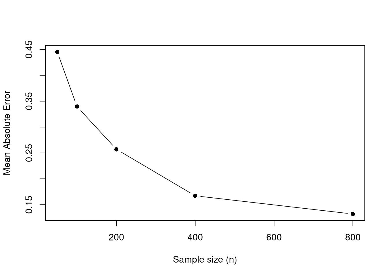
The simulation below illustrates this at one target point. The span is \(2n^{-1/5}\), which satisfies the same two conditions as \(n^{-1/5}\). The mean absolute error in estimating the population mean tends to decrease with larger \(n\).

## MAIN EXAMPLE
x_target <- 12 # high school graduates
n_grid <- c(50, 100, 200, 400, 800)
n_rep <- 200

avg_abs_err <- numeric(length(n_grid))
for (ni in seq_along(n_grid)) {
    n <- n_grid[ni]
    # The factor 2 keeps the span above 0.5 for these sample sizes.
    # About a third of workers have exactly 12 years of schooling.
    # Narrower spans can leave no other schooling level in the neighborhood.
    # Then loess() breaks down.
    span_n <- min(0.9, 2*n^(-1/5)) # shrinks with n
    errs <- replicate(n_rep, {
        xy_sim <- draw_xy(n)
        reg_lo <- loess(y_hat ~ x_hat, data=xy_sim, span=span_n, degree=1)
        y_pred <- predict(reg_lo, newdata=data.frame(x_hat=x_target))
        abs(y_pred - population_curve[as.character(x_target)])
    })
    avg_abs_err[ni] <- mean(errs, na.rm=TRUE)
}

plot(n_grid, avg_abs_err, type='b', pch=16,
     xlab='Sample size (n)',
     ylab='Mean Absolute Error',
     main=NA)

# The error falls from about 0.45 with 50 workers to about 0.13 with 800.

NoteMust Know

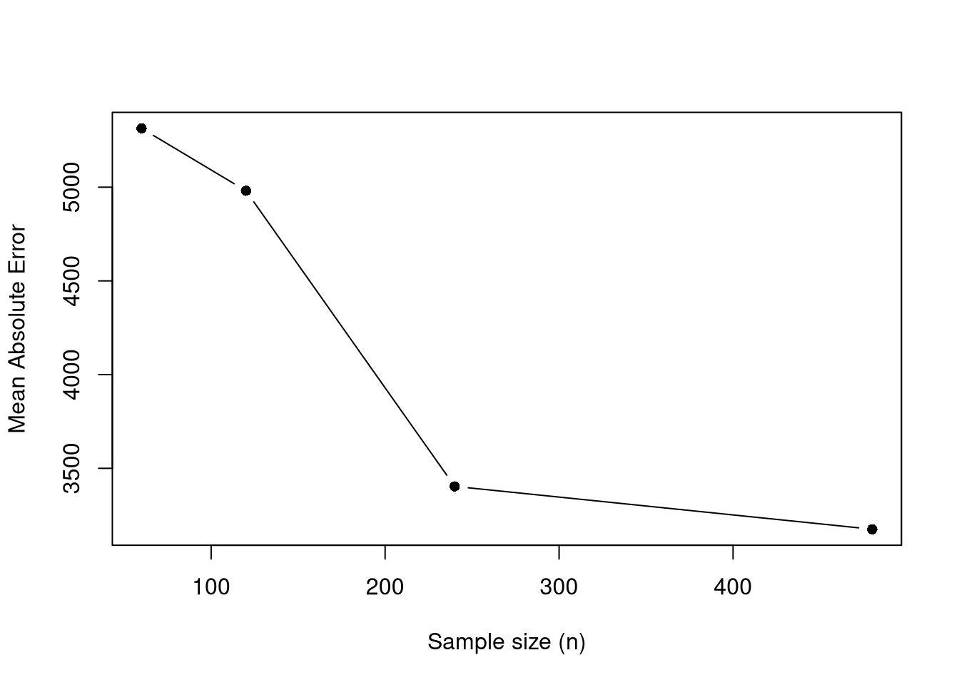
With a continuous \(\hat{x}\), the span can follow the rule \(h_{n}=n^{-1/5}\) directly, without the factor \(2\). Here yearly productivity depends on age through a smooth true mean, and we check the error at age \(40\).

# True mean productivity at each age
true_m <- function(x){
    m_x <- (1E-10*exp(1.4*x - .015*x^2)*x + 5E5) / 10
    return(m_x)
}

# Simulate n workers with ages evenly spaced from 15 to 70
sim_xy <- function(n){
    x_sim <- seq(15, 70, length.out=n)
    y_sim <- true_m(x_sim) + runif(n, -5E4, 5E4) # true mean plus noise
    return(data.frame(y_sim, x_sim))
}

x_target <- 40  # mid-career age
n_grid <- c(60, 120, 240, 480)
n_rep <- 120

avg_abs_err <- numeric(length(n_grid))
for (ni in seq_along(n_grid)) {
    n <- n_grid[ni]
    span_n <- min(0.9, n^(-1/5)) # shrinks with n
    errs <- replicate(n_rep, {
        xy_sim <- sim_xy(n)
        reg_lo <- loess(y_sim ~ x_sim, data=xy_sim, span=span_n, degree=1)
        y_pred <- predict(reg_lo, newdata=data.frame(x_sim=x_target))
        abs(y_pred - true_m(x_target))
    })
    avg_abs_err[ni] <- mean(errs, na.rm=TRUE)
}

plot(n_grid, avg_abs_err, type='b', pch=16,
    xlab='Sample size (n)',
    ylab='Mean Absolute Error',
    main=NA)

A similar result holds for OLS when the data come from a linear data generating process. Even with unlimited data, however, a misspecified model cannot recover the conditional expectation, as the linear fit to the pretend population shows.

19.3 Exercises

1. Comment the script you wrote for this chapter, then restart R and check that it runs from a clean session, then check the script with AI as explained in Working with AI. Write three sentences from memory on the main statistical idea of this chapter, and ask the assistant what is wrong, vague, or missing. Finish with your own questions about whatever you found hardest.

2. Using the USArrests dataset, regress Murder on UrbanPop with lm. Extract the theoretical \(t\)-statistic and \(p\)-value for the slope from summary(). Then write a bootstrap loop with \(B = 399\) replicates to compute a bootstrap \(p\)-value and compare it to the theoretical one.

3. A linear regression has low variance but can have high bias when the true relationship is nonlinear. A loess regression with a small span has low bias but high variance. Explain why increasing the sample size \(n\) helps reduce the standard error for both models, but only helps reduce bias for loess (with an appropriate bandwidth rule).

Further Reading

Many introductory econometrics textbooks have a good appendix on probability and statistics. See also the further reading in Bivariate Theory.

• https://www.econometrics-with-r.org/5-htaciam.html – hypothesis testing, Type I and Type II errors, and power in a regression context.
• https://learningstatisticswithr.com/book/regression.html#hypothesistestsforregressionmodels – testing regression slopes, interpreting p-values, and understanding standard errors.
• https://www.khanacademy.org/math/statistics-probability/significance-tests-one-sample/idea-of-significance-tests/v/simple-hypothesis-testing – video walkthrough of the logic behind hypothesis tests and p-values.
• https://www.khanacademy.org/computing/computer-science/informationtheory/moderninfotheory/v/bias-variance – visual introduction to the bias-variance tradeoff that drives bandwidth choice.

Recall

This chapter tested two means with Welch’s \(t\)-test and a regression slope with the theoretical \(t_{n-2}\) distribution. It also used the large-sample \(z\)-statistic, which covers a difference in medians as well. It then decomposed prediction error into squared bias and variance. The bootstrap for wages and schooling showed that the histogram of \(\hat{t}\) roughly matched the theoretical \(t_{n-2}\) density. Treating Wages1 as a known population, the linear fit predicted a mean wage of \(5.96\) at \(12\) years of schooling against a population mean of \(5.67\), a bias that more data does not remove, while the LOESS error was mostly variance that shrank as \(n\) grew.

McGill, Robert, John W. Tukey, and Wayne A. Larsen. 1978. “Variations of Box Plots.” The American Statistician 32 (1): 12–16. https://doi.org/10.1080/00031305.1978.10479236.

Satterthwaite, F. E. 1946. “An Approximate Distribution of Estimates of Variance Components.” Biometrics Bulletin 2 (6): 110–14. https://doi.org/10.2307/3002019.

Student. 1908. “The Probable Error of a Mean.” Biometrika 6 (1): 1–25. https://doi.org/10.2307/2331554.

Welch, B. L. 1947. “The Generalization of ‘Student’s’ Problem When Several Different Population Variances Are Involved.” Biometrika 34 (1-2): 28–35. https://doi.org/10.1093/biomet/34.1-2.28.

---

1. One benefit of local linear regression is that it is theoretically motivated. Suppose that \(Y_{i}=m_{Y}(X_{i}) + \epsilon_{i}\), where \(m_{Y}(x)\) is the population average of \(Y_{i}\) among observations with \(X_{i}=x\), and \(\epsilon_{i}\) is an unobserved random error that averages zero at each value of \(X_{i}\). For \(X_{i}\) near \(x\), a Taylor approximation gives \[\begin{aligned} m_{Y}(X_{i}) + \epsilon_{i} &\approx m_{Y}(x) + m_{Y}'(x)[X_{i}-x] + \epsilon_{i} \\ &= [m_{Y}(x) - m_{Y}'(x)x ] + m_{Y}'(x)X_{i} + \epsilon_{i} \\ &= b_{0}(x,h) + b_{1}(x,h) X_{i} + \epsilon_{i}. \end{aligned}\] So near \(x\), the population relationship is approximately a line with slope \(b_{1}(x,h)=m_{Y}'(x)\), which is what a local linear regression fits.