17  Local Regression II


Often, we are interested in gradients: how \(\hat{y}\) changes with \(\hat{x}\). The linear model from Simple Regression depicts this as a single constant, \(\hat{b}_{1}\), but the local-regression models from Local Regression do not. A great first step to assess gradients is to plot the predicted values over the explanatory values. A great second step is to compute gradients and summarize them.

This chapter asks three questions.

17.1 LOESS

Two problems with the local regressions from Local Regression motivate LOESS, which R fits with loess().

Code
## MAIN EXAMPLE
## Data: 3294 US workers, with hourly wages in 1980 dollars
data(Wages1, package='Ecdat')
xy_hat <- Wages1[order(Wages1[, 'school']), c('school', 'wage')]
colnames(xy_hat) <- c('x_hat', 'y_hat') # x_hat=years of schooling, y_hat=hourly wage

# Mean wage at each schooling level
school_means <- aggregate(y_hat ~ x_hat, data=xy_hat, mean)

Boundary Bias

The regressogram has a bias at the edges of the bins, which is addressed by the locally constant regression. Still, the locally constant regression has a bias near the edges of the dataset. Near the top of the data, the window around a design point can run past the largest \(\hat{x}_{i}\). So most of the observations in it have \(\hat{x}_{i}\) below the design point. The window average then describes a group centered below the design point. If \(\hat{y}\) rises with \(\hat{x}\), that average understates the mean of \(\hat{y}\) at the design point. The code below computes the window mean, a line fit to the same window, and the grouped mean at one such design point.

Code
# Locally constant fit near the top edge of the data
x <- 15 # design point
h <- 3.5 # window [11.5, 18.5] holds schooling levels 12 to 16
# The window runs past the most schooling anyone has, 16 years.
k_weights <- dunif( abs(xy_hat[, 'x_hat']-x)/h, -1, 1) # the uniform kernel k_U
xy_window <- xy_hat[k_weights > 0, ]
m_x <- mean(xy_window[, 'x_hat']) # average schooling in the window
m_y <- mean(xy_window[, 'y_hat']) # locally constant fit at x=15
c(m_x=m_x, m_y=m_y)
##       m_x       m_y 
## 12.686759  6.291988
# About 92 percent of workers in the window have under 15 years of schooling.
# So the window mean describes a group averaging about 12.7 years, not 15.

# A line fit to the same window, evaluated at the design point
reg_window <- lm(y_hat ~ x_hat, data=xy_window)
y_pred_line <- predict(reg_window, newdata=data.frame(x_hat=x))
y_pred_line
##        1 
## 8.244139
# The line follows the trend out to x=15, where it predicts about 8.24.

# Grouped mean wage at the design point
y_grp <- school_means[school_means[, 'x_hat'] == x, 'y_hat']
y_grp
## [1] 8.375111
# The window mean, about 6.29, sits far below the grouped mean of 8.38.
# Wages rise with schooling.
# So the window mean understates the mean wage at x=15.

# Plot the window
plot(y_hat ~ x_hat, data=xy_window, pch=16, col=grey(0, .1),
    ylim=c(0, 15), # zoom in on the fits
    main=NA, xlab='School', ylab='Wage')
abline(h=m_y, col=rgb(0, 0, 1, .8), lwd=2) # window mean
lines(c(12, 16), predict(reg_window, newdata=data.frame(x_hat=c(12, 16))),
    col=rgb(1, 0, 0, .8), lwd=2) # window line
points(m_x, m_y, pch=16, col=rgb(0, 0, 0, .8), cex=1.5) # window center
points(c(x, x), c(m_y, y_pred_line), pch=16, cex=1.5,
    col=c(rgb(0, 0, 1, .8), rgb(1, 0, 0, .8))) # the two fits at x=15
points(y_hat ~ x_hat, data=school_means, pch=24, col='white', bg=rgb(0, 0, 0, .8), cex=1.3) # grouped means
abline(v=x, col=grey(.5), lty=3)
legend('topleft',
    legend=c('Window mean', 'Window line', 'Window center', 'Grouped mean'),
    col=c(rgb(0, 0, 1, .8), rgb(1, 0, 0, .8), rgb(0, 0, 0, .8), 'white'),
    lty=c(1, 1, NA, NA), pch=c(NA, NA, 16, 24), lwd=2, pt.bg=rgb(0, 0, 0, .8), cex=.8, bg='white')
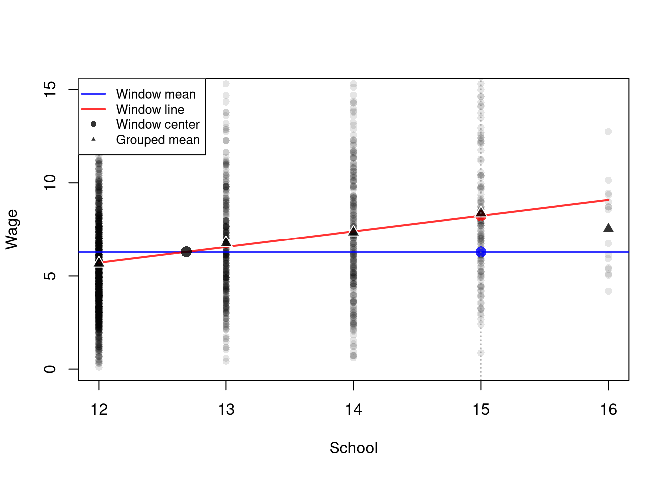
A line fit to the same window passes through the window center \((\hat{m}_{X}(x,h), \hat{m}_{Y}(x,h))\), just as the simple regression line passes through the point of means in Simple Linear Regression. Unlike the window mean, the line follows the trend out to the design point. So a local linear regression has less bias near the edges of the data.

Small Samples

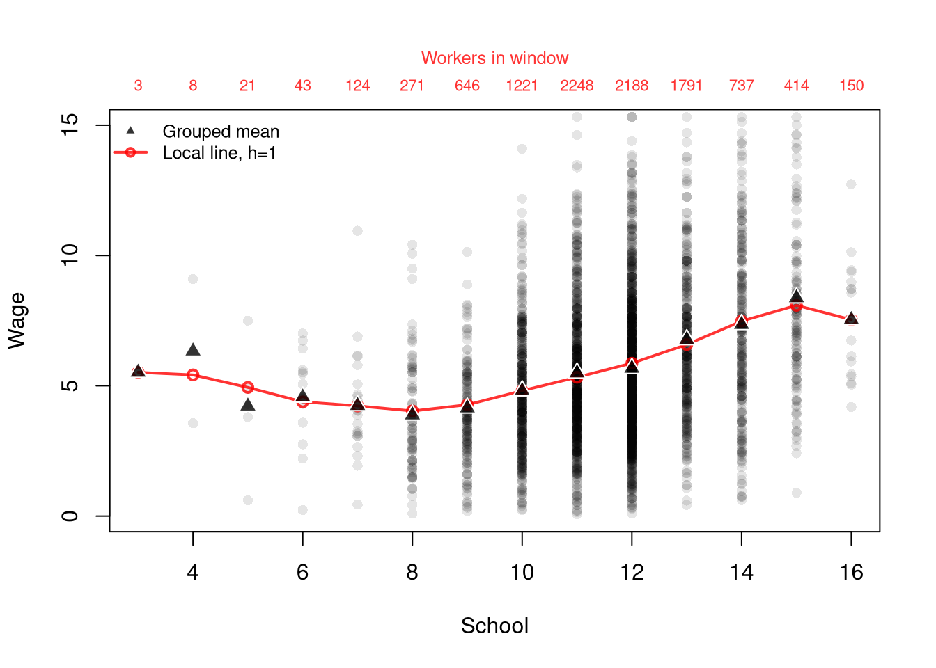
Another problem is that a fixed bandwidth gives each window a very different number of observations. Where the data are sparse, the windows are small samples. The code below fits a local line with \(h=1\) at every value of \(\hat{x}\) and counts the observations in each window.

Code
## MAIN EXAMPLE
# Fixed bandwidth: count the workers in each window and fit a line in it
x_values <- 3:16 # every schooling level
h <- 1 # each window holds three schooling levels
n_window <- rep(NA, length(x_values))
y_pred_fixed <- rep(NA, length(x_values))
for (i in seq_along(x_values)) {
    ki <- dunif( abs(xy_hat[, 'x_hat']-x_values[i])/h, -1, 1) # the uniform kernel k_U
    n_window[i] <- sum(ki > 0) # workers in the window
    reg_i <- lm(y_hat ~ x_hat, data=xy_hat, weights=ki) # weighted line
    y_pred_fixed[i] <- predict(reg_i, newdata=data.frame(x_hat=x_values[i]))
}
rbind(x=x_values, n_window=n_window)
##          [,1] [,2] [,3] [,4] [,5] [,6] [,7] [,8] [,9] [,10] [,11] [,12] [,13]
## x           3    4    5    6    7    8    9   10   11    12    13    14    15
## n_window    3    8   21   43  124  271  646 1221 2248  2188  1791   737   414
##          [,14]
## x           16
## n_window   150
# With h=1, the window at 3 years holds 3 workers and the one at 11 holds 2248.
# Few workers have fewer than 8 years of schooling or exactly 16 years.
# So the windows there are small samples.

# Raw data with the grouped means and the fitted line at each schooling level
# The workers in each window run along the top
plot(y_hat ~ x_hat, data=xy_hat, pch=16, col=grey(0, .1),
    ylim=c(0, 15), # zoom in on the fits, which hides the 43 highest wages
    main=NA, xlab='School', ylab='Wage')
lines(x_values, y_pred_fixed, col=rgb(1, 0, 0, .8), lwd=2, type='o')
points(y_hat ~ x_hat, data=school_means, pch=24, col='white', bg=rgb(0, 0, 0, .8), cex=1.3) # grouped means
axis(3, at=x_values, labels=n_window, tick=FALSE, line=-.5, cex.axis=.7, col.axis=rgb(1, 0, 0, .8))
mtext('Workers in window', side=3, line=1.5, cex=.8, col=rgb(1, 0, 0, .8))
legend('topleft', legend=c('Grouped mean', 'Local line, h=1'),
    pch=c(24, 1), lty=c(NA, 1), lwd=c(NA, 2), pt.bg=rgb(0, 0, 0, .8),
    col=c('white', rgb(1, 0, 0, .8)), cex=.8, bty='n')

Code
# The fitted wage falls from 3 to 8 years of schooling.
# The windows at 3, 4, and 5 years hold only 3, 8, and 21 workers.
# It also falls from 15 to 16 years, a dip set by the 16 workers with 16 years.

Fits in the smallest windows follow the few observations in them.

Adaptive Bandwidths

When \(\hat{x}_{i}\) is unevenly distributed across its range, a fixed bandwidth \(h\) leaves some local fits with many neighbors and others with very few.

ImportantKey Definition

LOESS (locally estimated scatterplot smoothing) fits a local linear (or quadratic) regression at each design point using an adaptive bandwidth (Cleveland 1979; Cleveland et al. 1988). Instead of fixing \(h\), it includes a fixed share of the data at each \(x\), set by the argument span. With a line in each window, the model for data near \(x\) is \[\begin{aligned} \hat{y}_{i} &= b_{0}(x) + b_{1}(x) \hat{x}_{i} + \hat{e}_{i}, \end{aligned}\] and the coefficients at \(x\) solve \[\min_{b_{0}(x), b_{1}(x)} \sum_{i=1}^{n}\left[\hat{y}_{i} - b_{0}(x) - b_{1}(x) \hat{x}_{i} \right]^{2} k\left(\hat{x}_{i}, x, h(x)\right),\] where the bandwidth \(h(x)\) is the distance from \(x\) to its \(q^{\text{th}}\) nearest \(\hat{x}_{i}\): \[\begin{aligned} h(x) &= \left|\hat{x}_{i}-x\right|_{(q)} \\ q &= \lfloor \text{span} \cdot n \rfloor. \end{aligned}\] Here \(|\hat{x}_{i}-x|_{(q)}\) is the \(q^{\text{th}}\) smallest of the distances \(|\hat{x}_{1}-x|, ..., |\hat{x}_{n}-x|\) and \(\lfloor \cdot \rfloor\) rounds down. The tricube kernel \[\begin{aligned} k\left(\hat{x}_{i}, x, h(x)\right) &= \left(1 - \frac{|\hat{x}_{i}-x|^{3}}{h(x)^{3}}\right)^{3} \end{aligned}\] weights observations with \(|\hat{x}_{i}-x| < h(x)\) and gives the rest weight \(0\).

LOESS is useful for smoothing data with uneven \(\hat{x}\). Because the share of points in each neighborhood is fixed, every window reaches the same number of nearest points, even where the data are sparse. The kernel weights still depend on distance, so the effective sample size can differ from window to window. The span argument plays the role \(h\) does for fixed-bandwidth methods, so smaller spans mean narrower neighborhoods, more flexibility, and noisier curves, while larger spans pool more data and smooth more aggressively.

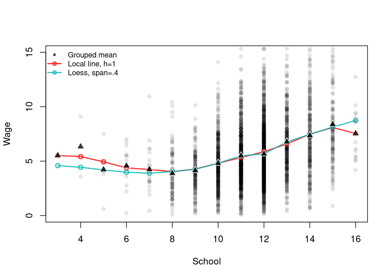
With degree=1, loess() fits a weighted line in each window, as the local linear regression does, so the main difference below is the window. We set span=.4, smaller than the default of \(0.75\), so the windows are narrower where the data are dense.

Code
## MAIN EXAMPLE
# Loess with a line in each window, so mainly the window differs from the fit above
reg_lo1 <- loess(y_hat ~ x_hat, data=xy_hat, degree=1, span=.4)
y_pred_lo1 <- predict(reg_lo1, newdata=data.frame(x_hat=x_values))

# Every window reaches the same number of nearest workers
floor(reg_lo1$pars$span*nrow(xy_hat))
## [1] 1317
# Each window reaches the 40 percent of workers nearest x, 1317 of the 3294.
# Schooling has ties, and workers exactly at the edge get zero weight.
# So at 3 years, only the 692 workers with under 11 years get positive weight.
# At 11, 12, and 13 years, only the workers at that level get positive weight.
# A line cannot be fit to one level, so loess() warns and its fit there is that level's mean.

# Compare the two fits
lo_col <- rgb(0, .7, .7, .8) # teal, the color of every LOESS fit
plot(y_hat ~ x_hat, data=xy_hat, pch=16, col=grey(0, .1),
    ylim=c(0, 15), # zoom in on the fits
    main=NA, xlab='School', ylab='Wage')
lines(x_values, y_pred_fixed, col=rgb(1, 0, 0, .8), lwd=2, type='o')
lines(x_values, y_pred_lo1, col=lo_col, lwd=2, type='o')
points(y_hat ~ x_hat, data=school_means, pch=24, col='white', bg=rgb(0, 0, 0, .8), cex=1.3) # grouped means
legend('topleft', legend=c('Grouped mean', 'Local line, h=1', 'Loess, span=.4'),
    pch=c(24, 1, 1), lty=c(NA, 1, 1), lwd=c(NA, 2, 2), pt.bg=rgb(0, 0, 0, .8),
    col=c('white', rgb(1, 0, 0, .8), lo_col), cex=.8, bty='n')

Code
# From 8 to 15 years, where workers are plentiful, the two fits differ by at most 20 cents.
# The loess fit does not follow the 3 workers with 3 or 4 years of schooling.
# It also does not follow the 16 workers with 16 years.
# The price is a much wider window: at 3 years, it reaches out to 11 years.

With span=.4, every LOESS window includes the \(40\) percent of observations nearest the design point. So the LOESS fit does not follow the few observations where the data are sparse. The price is a much wider window there.

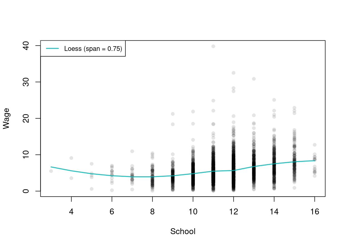
By default, loess() fits a local quadratic (degree=2) instead of a line, so the fitted curve can bend within each window. The rest of this chapter uses the default.

Code
## MAIN EXAMPLE
# Fit loess with the default span and degree
reg_lo <- loess(y_hat ~ x_hat, data=xy_hat)

A local quadratic adds the term \(b_{2}(x)\hat{x}_{i}^{2}\) in each window, so the coefficients at \(x\) solve \(\min_{b_{0}(x), b_{1}(x), b_{2}(x)} \sum_{i=1}^{n}\left[\hat{y}_{i} - b_{0}(x) - b_{1}(x) \hat{x}_{i} - b_{2}(x)\hat{x}_{i}^{2} \right]^{2} k\left(\hat{x}_{i}, x, h(x)\right)\).

Code
# reg_lo defined above
plot(y_hat ~ x_hat, pch=16, col=grey(0, .1), data=xy_hat,
    main=NA, xlab='School', ylab='Wage')
lines(xy_hat[, 'x_hat'], predict(reg_lo),
    col=lo_col, lwd=2)

legend('topleft',
    legend=sprintf('Loess (span = %.2f)', reg_lo$pars$span),
    lty=1, lwd=2, col=lo_col, cex=.8)

17.2 Model Fit

Each model produces fitted values \(\hat{y}_{i}^{\mathrm{fit}}\) and residuals \(\hat{e}_{i} = \hat{y}_{i} - \hat{y}_{i}^{\mathrm{fit}}\). To compare models, we often summarize the residuals with a single number.

The mean squared error averages the squared residuals, \[\begin{aligned} \hat{\text{MSE}} &= \frac{1}{n}\sum_{i=1}^{n} \hat{e}_{i}^2 = \frac{1}{n}\sum_{i=1}^{n} \left(\hat{y}_{i} - \hat{y}_{i}^{\mathrm{fit}}\right)^2. \end{aligned}\] Squaring penalizes large misses heavily, and the units are the square of the units of \(\hat{y}_{i}\).

The R-squared rescales \(\hat{\text{MSE}}\) by the variance of \(\hat{y}\), \[\begin{aligned} \hat{R}^{2} &= 1 - \frac{\hat{\text{RSS}}}{\hat{\text{TSS}}} = 1 - \frac{\hat{\text{MSE}}}{\hat{v}_{Y}}. \end{aligned}\] It is unit-free and applies to any model with fitted values. On the same data, it ranks models exactly as \(\hat{\text{MSE}}\) does. For least squares fits with an intercept, it also equals the squared correlation between \(\hat{y}_{i}\) and \(\hat{y}_{i}^{\mathrm{fit}}\). For any model, this squared correlation is the generalized \(R^{2}\) statistic, \[\begin{aligned} \hat{R}^{2}_{\text{gen}} &= \hat{r}_{YY^{\mathrm{fit}}}^{2} = \frac{\hat{c}_{YY^{\mathrm{fit}}}^{2}}{\hat{v}_{Y} \hat{v}_{Y^{\mathrm{fit}}}}, \end{aligned}\] where \(\hat{c}_{YY^{\mathrm{fit}}}\) is the covariance of \(\hat{y}\) and \(\hat{y}^{\mathrm{fit}}\), and \(\hat{v}_{Y^{\mathrm{fit}}}\) is the variance of \(\hat{y}^{\mathrm{fit}}\). For other fits, such as LOESS, the two versions can differ, and only \(\hat{R}^{2}_{\text{gen}}\) is guaranteed to lie between \(0\) and \(1\). Both estimate the share of the variation in \(Y_{i}\) that \(X_{i}\) explains (Doksum and Samarov 1995).

Suppose three workers have wages \(\hat{y}=(8, 10, 15)\) and a model predicts \(\hat{y}^{\mathrm{fit}}=(9, 9, 14)\). The residuals are \(\hat{e}=(-1, 1, 1)\), so \[\begin{aligned} \hat{\text{MSE}} &= \frac{(-1)^2 + 1^2 + 1^2}{3} = \frac{3}{3} = 1. \end{aligned}\] The model misses by \(1\) squared-dollar on average.

Code
y0_hat <- c(8, 10, 15)
y0_fit <- c(9, 9, 14)
e0_hat <- y0_hat - y0_fit
mean(e0_hat^2) # MSE
## [1] 1

We can compute these for the linear model, the regressogram with three bins, and LOESS.

Code
## MAIN EXAMPLE
# xy_hat and reg_lo defined above

# Two more models for wage on schooling
reg_lin <- lm(y_hat ~ x_hat, data=xy_hat)        # globally linear
xy_hat[, 'xcf'] <- cut(xy_hat[, 'x_hat'], 3)
reg_rgram <- lm(y_hat ~ xcf, data=xy_hat)         # regressogram, 3 bins

# Mean squared error and both R-squared statistics
fit_stats <- function(model){
    e_hat <- resid(model)
    y_hat <- xy_hat[, 'y_hat']
    c(MSE=mean(e_hat^2),
        R2=1 - mean(e_hat^2)/mean((y_hat-mean(y_hat))^2),
        R2_gen=cor(y_hat, y_hat-e_hat)^2)
}
fit_table <- rbind(
    Linear       = fit_stats(reg_lin),
    Regressogram = fit_stats(reg_rgram),
    LOESS        = fit_stats(reg_lo))
round(fit_table, 3)
##                 MSE    R2 R2_gen
## Linear        9.832 0.080  0.080
## Regressogram 10.270 0.039  0.039
## LOESS         9.721 0.090  0.090
# MSE is in squared dollars.
# LOESS has the smallest MSE, and the regressogram has the largest.
# Every R-squared is below 0.1.
# So each model leaves over 90 percent of the variation in wages unexplained.

A smaller error on the data used to fit a model does not guarantee smaller errors on new data, since a flexible enough model also fits the noise in the sample.

The mean absolute percentage error averages each residual relative to its observed value, \[\begin{aligned} \hat{\text{MAPE}} &= \frac{100}{n}\sum_{i=1}^{n} \left| \frac{\hat{e}_{i}}{\hat{y}_{i}} \right|. \end{aligned}\] MAPE is unit-free, which makes it easy to communicate, but it is undefined when \(\hat{y}_{i}=0\) and over-weights observations with small \(\hat{y}_{i}\). MSE is easier to analyze theoretically.

Compute \(\hat{\text{MAPE}}\) for the three workers with wages \(\hat{y}=(8, 10, 15)\) and predictions \(\hat{y}^{\mathrm{fit}}=(9, 9, 14)\). Then compute it for the line, the regressogram, and LOESS, and check whether it ranks the models as \(\hat{\text{MSE}}\) does.

For the three workers, the residuals are \(\hat{e}=(-1, 1, 1)\), so \[\begin{aligned} \hat{\text{MAPE}} &= \frac{100}{3}\left( \frac{1}{8} + \frac{1}{10} + \frac{1}{15} \right) = \frac{100}{3}\left( \frac{15}{120} + \frac{12}{120} + \frac{8}{120} \right) \\ &= \frac{100}{3} \times \frac{35}{120} = \frac{175}{18} \approx 9.7. \end{aligned}\] The model misses by about \(10\%\) of each wage.

Code
# y0_hat and e0_hat defined above
100*mean(abs(e0_hat/y0_hat))
## [1] 9.722222

# reg_lin, reg_rgram, and reg_lo defined above
mape <- function(model){
    100*mean(abs(resid(model)/xy_hat[, 'y_hat']))
}
round(c(Linear=mape(reg_lin), Regressogram=mape(reg_rgram), LOESS=mape(reg_lo)), 3)
##       Linear Regressogram        LOESS 
##       73.275       75.879       72.952
# LOESS has the smallest MAPE and the regressogram the largest, as with MSE.
# Every model misses by over 70 percent on average.
# Partly that is because a few workers earn less than 20 cents an hour.
# Their percentage errors are huge.

The two measures can rank models differently, because MAPE weights observations with low \(\hat{y}_{i}\) more heavily.

Adamson (2025) tests whether a more flexible model’s gain in fit is larger than chance, using a loss-in-fit statistic (Härdle and Mammen 1993; Henderson and Parmeter 2015). The statistic is the rise in the residual sum of squares from an unrestricted to a restricted model, divided by the unrestricted residual sum of squares. It is a nonparametric analog of the \(F\)-statistic, and the paper computes its \(p\)-values with a bootstrap.

Cross-Validation

To measure out-of-sample fit, we use the leave-one-out cross-validation error \(\hat{\text{CV}}\), the \(\hat{\text{MSE}}\) of predictions for held-out observations. A model that fits the noise in the sample predicts held-out observations poorly, so its \(\hat{\text{CV}}\) rises above its \(\hat{\text{MSE}}\).

The code below refits each model \(n\) times, each time without one observation, and predicts that observation’s \(\hat{y}_{i}\).

Code
## MAIN EXAMPLE
# xy_hat defined above, including the bins xcf

# Leave-one-out prediction errors, one column per model
loo_errors <- matrix(NA, nrow=nrow(xy_hat), ncol=3)
colnames(loo_errors) <- c('Linear', 'Regressogram', 'LOESS')
loo_errors_mean <- rep(NA, nrow(xy_hat))
for (i in seq_len(nrow(xy_hat))) {
    xy_i <- xy_hat[-i, ] # drop worker i
    reg_lin_i   <- lm(y_hat ~ x_hat, data=xy_i)
    reg_rgram_i <- lm(y_hat ~ xcf, data=xy_i)
    reg_lo_i    <- loess(y_hat ~ x_hat, data=xy_i)
    # Predict worker i from the fits without worker i
    y_pred_i <- c(
        predict(reg_lin_i, newdata=xy_hat[i, ]),
        predict(reg_rgram_i, newdata=xy_hat[i, ]),
        predict(reg_lo_i, newdata=xy_hat[i, ]))
    loo_errors[i, ] <- xy_hat[i, 'y_hat'] - y_pred_i
    # Compare worker i with the mean wage of the other workers
    loo_errors_mean[i] <- xy_hat[i, 'y_hat'] - mean(xy_i[, 'y_hat'])
}

# LOESS does not extrapolate, so it cannot predict the only worker with 3 years of schooling
# Compare all models on the workers every model can predict
loo_ok <- complete.cases(loo_errors)
cv_hat <- colMeans(loo_errors[loo_ok, ]^2)

# Out-of-sample R-squared rescales CV by the leave-one-out version of the variance, for the same workers
v_cv_hat <- mean(loo_errors_mean[loo_ok]^2)
r2_cv <- 1 - cv_hat/v_cv_hat

# Out-of-sample generalized R-squared squares the correlation of wages and held-out predictions
y_ok <- xy_hat[loo_ok, 'y_hat']
y_pred_cv <- y_ok - loo_errors[loo_ok, ]
r2_gen_cv <- cor(y_ok, y_pred_cv)[1, ]^2
round(cbind(fit_table, CV=cv_hat, R2_CV=r2_cv, R2_gen_CV=r2_gen_cv), 3)
##                 MSE    R2 R2_gen     CV R2_CV R2_gen_CV
## Linear        9.832 0.080  0.080  9.840 0.080     0.079
## Regressogram 10.270 0.039  0.039 10.288 0.038     0.037
## LOESS         9.721 0.090  0.090  9.762 0.087     0.087
# Every model predicts held-out workers a little worse than those it was fit to.
# The gap between CV and MSE grows with flexibility.
# It runs from about 0.01 for the line to about 0.04 for LOESS.
# LOESS still predicts held-out workers best.
# Its lead over the line shrinks from about 0.11 in sample to about 0.08.
# R2_gen_CV falls below its in-sample version for every model.
# R2_CV also falls, except that the line's rounds to its in-sample R-squared.
# That is because R2_CV omits the one worker LOESS cannot predict.
# R2_CV and R2_gen_CV are within about 0.001 of each other.
# They differ more for the USArrests line in Simple Regression (not run here).
# Its R2_CV is negative, about -0.04, yet its R2_gen_CV is about 0.22.
# That is above its in-sample R-squared of about 0.005.
# Squaring hides the sign of the correlation, which is about -0.47.

The gap between \(\hat{\text{CV}}\) and \(\hat{\text{MSE}}\) tends to grow with a model’s flexibility. The out-of-sample generalized \(R^{2}\) replaces the fitted values in \(\hat{R}^{2}_{\text{gen}}\) with the held-out predictions \(\hat{y}^{\mathrm{pred}(-i)}(\hat{x}_{i})\), \[\begin{aligned} \hat{R}^{2}_{\text{gen,CV}} &= \hat{r}_{YY^{\mathrm{pred}(-i)}}^{2}, \end{aligned}\] where \(\hat{r}_{YY^{\mathrm{pred}(-i)}}\) is the correlation between \(\hat{y}_{i}\) and \(\hat{y}^{\mathrm{pred}(-i)}(\hat{x}_{i})\). The out-of-sample R-squared \(\hat{R}^{2}_{\text{CV}}\) is negative when a model predicts held-out observations worse than the mean of the other observations would, but \(\hat{R}^{2}_{\text{gen,CV}}\) always lies between \(0\) and \(1\). The two can differ, since a squared correlation ignores whether the predictions are shifted or scaled away from the observed \(\hat{y}_{i}\). Squaring also hides a negative correlation, so a model can have an \(\hat{R}^{2}_{\text{gen,CV}}\) above its in-sample \(\hat{R}^{2}\) even when its \(\hat{R}^{2}_{\text{CV}}\) is negative, as a Test Yourself in Cross-Validation shows.

Adamson (2025) compares a locally constant regression with a linear model using both in-sample and out-of-sample errors (Mullainathan and Spiess 2017). It notes that fitting simple models to complex relationships is believed to be a major source of false positives (Henderson and Parmeter 2015; Racine 2019; Hansen 2022).

17.3 Gradients

Once the fitted curve can bend, “the slope” is no longer a single number; we want the slope locally at each \(x\).

ImportantKey Definition

A gradient \(\hat{b}_{1}(x)\) at the design point \(x\) is the rate of change of the prediction \(\hat{y}^{\mathrm{pred}}(x)\) with respect to \(x\) in a neighborhood of \(x\).

The mean of the gradients (sometimes called the average effect or mean marginal effect) averages \(\hat{b}_{1}(x)\) across every observation in the dataset: \[\frac{1}{n}\sum_{i=1}^{n} \hat{b}_{1}(x=\hat{x}_{i}).\]

The gradient is useful as the local analog of the simple-regression slope. For a globally linear model, it equals the single coefficient \(\hat{b}_{1}\) everywhere. For a local model, it varies with \(x\) and shows how the marginal relationship changes across the range of \(\hat{x}\). Three common ways to estimate gradients are:

  1. For all methods, including regressograms, you can approximate gradients with small finite differences. For some small difference \(d\), we can manually compute \[\begin{aligned} \hat{b}_{1}(x) &= \frac{ \hat{y}^{\mathrm{pred}}(x+\frac{d}{2}) - \hat{y}^{\mathrm{pred}}(x-\frac{d}{2})}{d}, \end{aligned}\]

  2. When using split-sample regressions or local linear regressions, you can use the estimated slope coefficients \(\hat{b}_{1}(x)\) as a gradient estimate.

  3. More sophisticated methods that are beyond the scope of this book.

Suppose a local model predicts wages near \(x=12\) years of schooling: \(\hat{y}^{\mathrm{pred}}(11.5)=9.2\) and \(\hat{y}^{\mathrm{pred}}(12.5)=10.4\) (dollars per hour). With step \(d=1\), the finite-difference gradient at \(x=12\) is \[ \hat{b}_{1}(12) = \frac{\hat{y}^{\mathrm{pred}}(12.5) - \hat{y}^{\mathrm{pred}}(11.5)}{d} = \frac{10.4 - 9.2}{1} = 1.2. \] Near \(12\) years of schooling, each extra year is associated with about \(\$1.20\) more per hour.

Code
d <- 1
y_pred_hi <- 10.4  # prediction at x + d/2
y_pred_lo <- 9.2   # prediction at x - d/2
(y_pred_hi - y_pred_lo) / d
## [1] 1.2

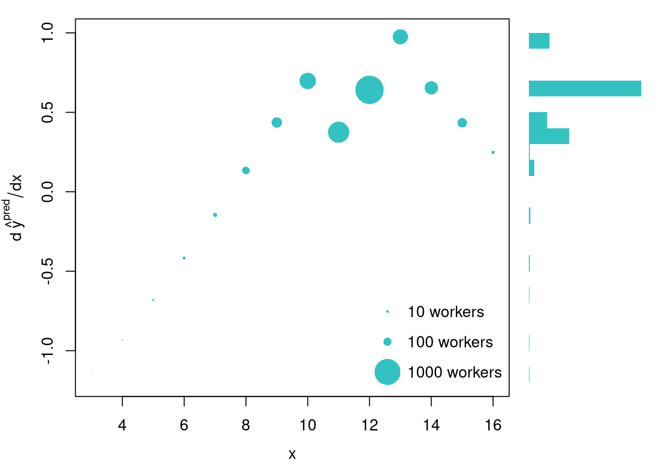
After computing gradients, you can summarize them in various plots, such as histograms and scatterplots. These plots show how the gradient varies within the sample. You can also plot all gradients with their confidence intervals (Chaudhuri and Marron 1999; Henderson et al. 2012).

Code
## MAIN EXAMPLE
## Gradient at each observation, as a centered finite difference with d=1
## Many workers share a schooling level, so compute it once per level
grad_by_obs <- function(xy, reg, d=1) {
    x_levels <- sort(unique(xy[, 'x_hat']))
    # loess does not extrapolate, so the step is cut short at the edges of the data
    x_lo <- pmax(x_levels - d/2, min(x_levels))
    x_hi <- pmin(x_levels + d/2, max(x_levels))
    y_pred_lo <- predict(reg, newdata=data.frame(x_hat=x_lo))
    y_pred_hi <- predict(reg, newdata=data.frame(x_hat=x_hi))
    grad_levels <- (y_pred_hi - y_pred_lo)/(x_hi - x_lo)
    grad_obs <- grad_levels[match(xy[, 'x_hat'], x_levels)]
    return(grad_obs)
}
grad_obs <- grad_by_obs(xy_hat, reg_lo)

## Visual Summary
f_grad <- hist(grad_obs, breaks=20, plot=FALSE)
layout(matrix(1:2, ncol=2), widths=c(4/5, 1/5))

# One point per schooling level, since all workers at a level share one gradient
x_levels <- sort(unique(xy_hat[, 'x_hat']))
grad_levels <- grad_obs[match(x_levels, xy_hat[, 'x_hat'])]
n_levels <- as.numeric(table(xy_hat[, 'x_hat']))

# Point area scales with the number of workers
sizes <- sqrt(n_levels / max(n_levels)) * 4

# Scatterplot, with limits that line up with the marginal bars below
par(mar=c(4, 4, 1, 1))
plot(x_levels, grad_levels, cex=sizes,
    xlab='x', ylab=expression(d~hat(y)^plain(pred)/dx),
    mgp=c(2.5, 1, 0),
    ylim=range(f_grad[['breaks']]),
    col=lo_col, pch=16, main=NA) ## Diminishing Returns?
legend('bottomright', bty='n', y.intersp=1.6, x.intersp=1.4,
    legend=c('10 workers', '100 workers', '1000 workers'),
    pch=16, col=lo_col, pt.cex=sqrt(c(10, 100, 1000) / max(n_levels)) * 4)

# Add Marginal
par(mar=c(4, 0, 1, 1))
barplot(f_grad[['density']], axes=FALSE, space=0, horiz=TRUE, border=NA,
    col=lo_col) ## Distributional Summary

Code
# The largest point is at 12 years, where 1188 workers share one gradient.
# The longest bar, gradients from 0.6 to 0.7, holds the 1851 workers with 10, 12, or 14 years.
# Only the 46 workers with under 8 years of schooling have negative gradients.

A different kind of summary collapses the whole gradient curve into a single number for tabular reporting. The mean of the gradients answers “what is the average slope across the sample?”. This generally differs from the gradient at the mean (sometimes called the marginal effect at the mean) which evaluates the gradient at a single design point: \(\hat{b}_{1}(x=\hat{m}_{X})\) and answers “what is the slope at a typical \(\hat{x}_{i}\)?” The two coincide for a globally linear model but can differ for any other, sometimes substantially when the relationship bends (Henderson et al. 2012; Adamson 2021). You may also be interested in the median of the gradients, or in measures of effect heterogeneity like the interquartile range or standard deviation of the gradients. Such statistics can be presented in tabular form with estimates of sampling variability.

These two summaries usually differ. Suppose a local model has gradients \(\hat{b}_{1}(x)\) at schooling levels \(x=(8,10,12,14,16)\) equal to \((0.4, 0.8, 1.2, 0.9, 0.3)\), and the sample mean schooling is \(\hat{m}_{X}=12\).

  • The gradient at the mean is the single gradient at \(x=\hat{m}_{X}\): \(\hat{b}_{1}(12) = 1.2\).
  • The mean of the gradients averages over all five points: \(\frac{0.4+0.8+1.2+0.9+0.3}{5} = \frac{3.6}{5} = 0.72\).

They differ because the gradient is not constant: here the relationship is steepest near the mean and flatter at the extremes.

Code
grads <- c(0.4, 0.8, 1.2, 0.9, 0.3)
grads[3]      # gradient at the mean (x = 12)
## [1] 1.2
mean(grads)   # mean of the gradients
## [1] 0.72

The code below computes the gradient at the mean, along with the mean and the standard deviation of the gradients.

Code
## MAIN EXAMPLE
## Gradient at the mean, as a centered finite difference with d=1 around the mean schooling
grad_at_mean <- function(xy, reg, d=1) {
    m_hat <- mean(xy[, 'x_hat'])
    y_pred_d <- predict(reg, newdata=data.frame(x_hat=c(m_hat-d/2, m_hat+d/2)))
    grad_m <- (y_pred_d[2] - y_pred_d[1])/d
    return(unname(grad_m))
}

## Tabular Summary
## grad_obs defined above
tab_stats <- c(
    'At the mean'=grad_at_mean(xy_hat, reg_lo),
    Mean=mean(grad_obs),
    SD=sd(grad_obs))
round(tab_stats, 3)
## At the mean        Mean          SD 
##       0.239       0.583       0.220
# The gradient at the mean, about 0.24, is much smaller than the mean gradient.
# The mean of the gradients is about 0.58.
# The mean schooling, about 11.6 years, falls between 11 and 12 years.
# The loess curve is flatter there than at the neighboring levels.

17.4 Variability Estimates

Confidence Bands

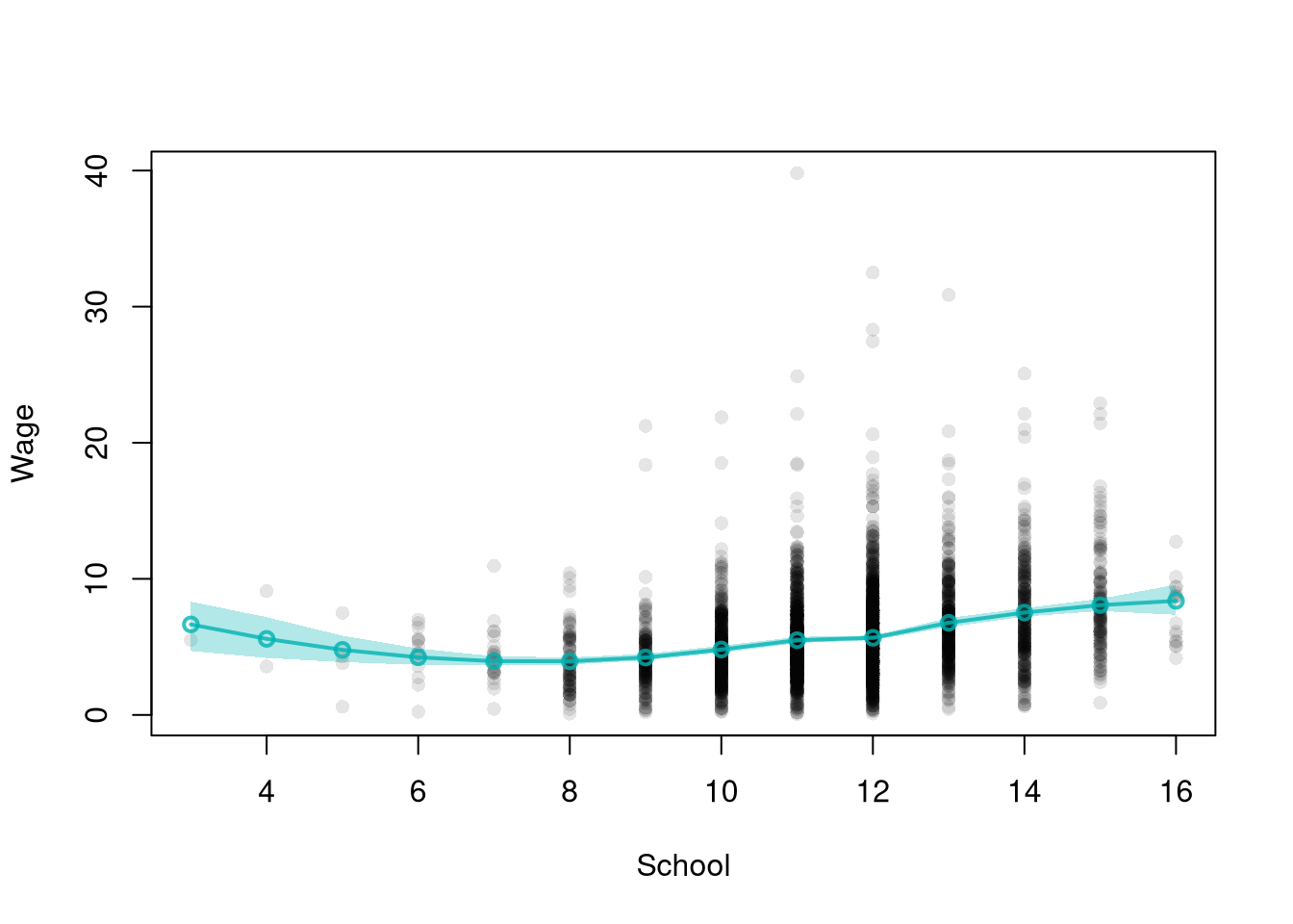
A single fitted curve does not show how much that curve would change in another sample, so we draw a region around it.

ImportantKey Definition

A confidence band is a confidence interval drawn at every design point: a region around the fitted curve that captures sample-to-sample variability. A bootstrap confidence band collects the predictions from many resamples and reads off pointwise quantiles at each \(x\).

Confidence bands are useful for showing where a fitted curve is well-supported by the data and where another sample could move it. The width is typically wider at the edges of \(\hat{x}\) (few neighbors) and narrower in the dense middle, which is itself a quick visual diagnostic. The same bootstrap that produces the band also produces standard errors for any single design point and for the gradient summaries below. The band shows variability across samples, whereas the gradient plots show variability within the sample.

Code
## MAIN EXAMPLE
# Same loess fit as above (default span)
pred_design <- data.frame(x_hat=unique(xy_hat[, 'x_hat']))
y_pred <- predict(reg_lo, newdata=pred_design)

plot(y_hat ~ x_hat, pch=16, col=grey(0, .1), data=xy_hat,
    main=NA, xlab='School', ylab='Wage')
lines(pred_design[, 'x_hat'], y_pred,
    col=lo_col, lwd=2, type='o')

# Boot CI with the same default-span loess
boot_lo <- matrix(NA, nrow=nrow(pred_design), ncol=399)
for (b in 1:399) {
    xy_boot <- xy_hat[sample(nrow(xy_hat), replace=TRUE), ]
    reg_b <- loess(y_hat ~ x_hat, data=xy_boot)
    boot_lo[, b] <- predict(reg_b, newdata=pred_design)
}
boot_cb <- apply(boot_lo, 1, quantile,
    probs=c(.025, .975), na.rm=TRUE)

# Plot CI
polygon(
    c(pred_design[[1]], rev(pred_design[[1]])),
    c(boot_cb[1, ], rev(boot_cb[2, ])),
    col=rgb(0, .7, .7, .3),
    border=NA)

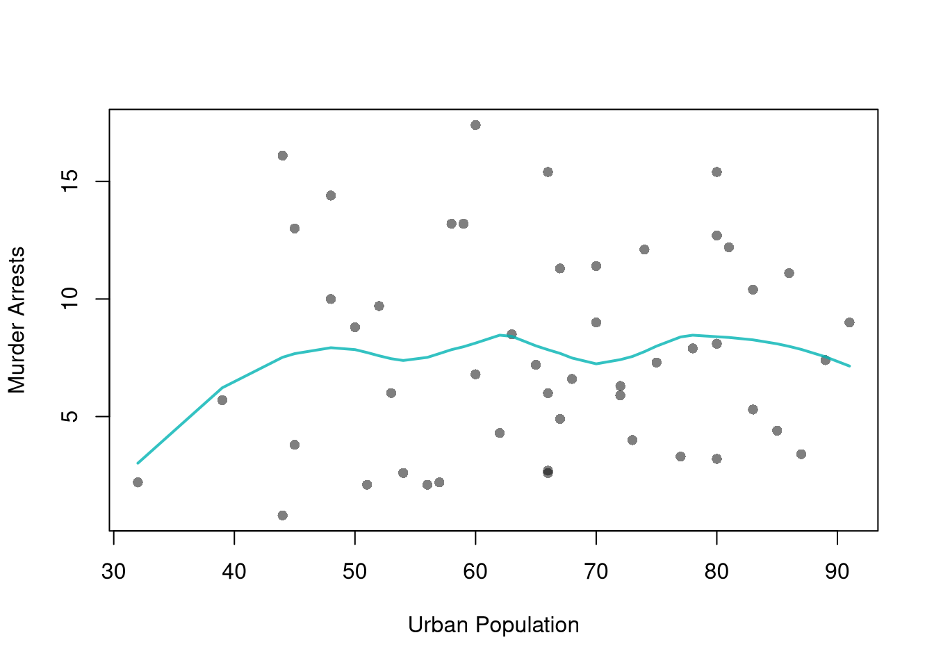
Construct a bootstrap confidence band for the following loess regression

Code
# Adaptive-width subsamples with non-uniform weights
xy2_hat <- USArrests[, c('UrbanPop', 'Murder')]
colnames(xy2_hat) <- c('x_hat', 'y_hat') # x_hat=urban population share, y_hat=murder arrests per 100K
xy2_ord_hat <- xy2_hat[order(xy2_hat[, 'x_hat']), ]

plot(y_hat ~ x_hat, pch=16, col=grey(0, .5), data=xy2_ord_hat,
    main=NA, xlab='Urban Population', ylab='Murder Arrests')
reg_lo_usa <- loess(y_hat ~ x_hat, data=xy2_ord_hat, span=.6)

lines(xy2_ord_hat[, 'x_hat'], predict(reg_lo_usa),
    col=lo_col, lwd=2)

Gradient Standard Errors

Repeating the gradient summaries on each bootstrap resample gives their standard errors and confidence intervals.

Code
## MAIN EXAMPLE
## Use bootstrap to approximate sampling dist
boot_stats <- matrix(NA, nrow=299, ncol=3)
colnames(boot_stats) <- c('At the mean', 'Mean', 'SD')
for(b in 1:nrow(boot_stats)){
    xy_boot <- xy_hat[sample(1:nrow(xy_hat), replace=TRUE), ]
    reg_lo_b <- loess(y_hat ~ x_hat, data=xy_boot)
    grad_m_b_hat <- grad_at_mean(xy_boot, reg_lo_b)
    grad_obs_b <- grad_by_obs(xy_boot, reg_lo_b)
    m_grad_b_hat <- mean(grad_obs_b)
    s_grad_b_hat <- sd(grad_obs_b)
    boot_stats[b, 1] <- grad_m_b_hat
    boot_stats[b, 2] <- m_grad_b_hat
    boot_stats[b, 3] <- s_grad_b_hat
}
## SEs and CIs
boot_se <- apply(boot_stats, 2, sd)
boot_quants <- apply(boot_stats, 2, quantile, probs=c(0.025, 0.975))
boot_quants <- apply( round(boot_quants, 3), 2, paste0, collapse=', ')

## Printing
tab_regstyle <- data.frame(
  Estimate  = round(tab_stats, 3),
  SE = paste0('(', round(boot_se, 3), ')'),
  CI_95 = paste0('[', boot_quants, ']')
)
tab_regstyle
##             Estimate      SE          CI_95
## At the mean    0.239  (0.15) [-0.046, 0.53]
## Mean           0.583 (0.047)  [0.49, 0.667]
## SD             0.220 (0.045) [0.176, 0.363]
# The gradient at the mean varies more across samples: its SE is about 0.15.
# The SE of the mean of the gradients is about 0.047.
# The interval for the gradient at the mean includes zero.
# The interval for the mean of the gradients does not.
Summary of Local Gradients
Estimate Bootstrap SE Bootstrap 95% CI
At the mean 0.239 (0.15) [-0.046, 0.53]
Mean 0.583 (0.047) [0.49, 0.667]
SD 0.220 (0.045) [0.176, 0.363]

The gradient at the mean depends on the fit near a single design point, so it tends to vary more across samples than the mean of the gradients, which averages over all observations.

17.5 Hypothesis Testing

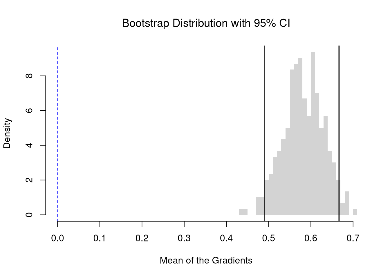
We can test whether the mean gradient is statistically different from zero. The first way is to invert a confidence interval. A \(95\%\) confidence interval gives a test at the \(5\%\) level: reject a hypothesized value if it falls outside the interval, and fail to reject it if it falls inside. So we need no new resampling to test \(H_{0}\): the mean gradient equals zero. We only check whether the bootstrap interval from Gradient Standard Errors contains \(0\).

Code
## MAIN EXAMPLE
## Bootstrap distribution of the mean gradient, with its 95% CI and zero marked
## boot_stats defined above
boot_ci_mean <- quantile(boot_stats[, 'Mean'], probs=c(.025, .975))

hist(boot_stats[, 'Mean'], breaks=25,
    border=NA, freq=FALSE,
    xlim=range(c(0, boot_stats[, 'Mean'])),
    xlab='Mean of the Gradients',
    main=NA)
title('Bootstrap Distribution with 95% CI', font.main=1)
abline(v=boot_ci_mean, col=rgb(0, 0, 0, .8), lwd=2) # 95% CI
abline(v=0, col=rgb(0, 0, 1, .8), lty=2)            # H0: mean gradient=0

Code

## Does the 95% interval contain zero?
boot_ci_mean
##      2.5%     97.5% 
## 0.4902400 0.6667944
unname(boot_ci_mean[1] <= 0 & boot_ci_mean[2] >= 0)
## [1] FALSE
# The interval, about 0.49 to 0.67, does not contain 0.
# So we reject the null that the mean gradient is zero at the 5% level.
# The interval for the gradient at the mean, about -0.05 to 0.53, does contain 0.
# So we fail to reject the same null for that statistic.

We can also compute the p-value directly from the same bootstrap distribution. Under \(H_{0}\), the mean gradient equals zero, so we center the bootstrap distribution at zero, as in Impose the Null, and ask how often it produces values as extreme as the observed mean gradient.

Code
## MAIN EXAMPLE
## P-value via null bootstrap
## Center bootstrap means at zero (impose H0)
boot_centered <- boot_stats[, 'Mean'] - mean(boot_stats[, 'Mean'])

## Two-sided p-value: P(|centered mean| >= |observed mean|)
p_boot <- mean(abs(boot_centered) >= abs(tab_stats['Mean']))

cat('Bootstrap p-value:', p_boot, '\n')
## Bootstrap p-value: 0
# The observed mean gradient is farther from zero than all 299 centered means.
# So the p-value is 0.
# That only says the p-value is probably below about 3/299, or 0.01.
# The mean gradient is statistically distinguishable from zero.
# On average, wages increase with schooling.

With \(B\) resamples, a p-value of \(0\) means only that no resample was as extreme as the observed statistic. The p-value with unlimited resamples could still be about \(3/B\), which would produce no such resample about \(5\%\) of the time. A small p-value indicates that the mean gradient is statistically distinguishable from zero.

We can also use a normal approximation. Under the null hypothesis \(H_{0}\): the mean gradient equals zero, we use the test statistic \[\hat{t} = \frac{\text{mean gradient}}{\hat{\text{SE}}(\text{mean gradient})}\] and the p-value comes from the standard normal distribution.

Code
## P-value for mean gradient
## Standard Normal Approximation
t_stat <- tab_stats['Mean'] / boot_se['Mean']
p_val  <- 2 * pnorm(-abs(t_stat))

cat('Mean gradient:', round(tab_stats['Mean'], 3), '\n')
## Mean gradient: 0.583
cat('Bootstrap SE: ', round(boot_se['Mean'], 3), '\n')
## Bootstrap SE:  0.047
cat('t-statistic:  ', round(t_stat, 3), '\n')
## t-statistic:   12.372
cat('p-value:      ', format.pval(p_val, digits=3), '\n')
## p-value:       <2e-16

Compute the t-statistic and p-value using jackknife standard errors instead of the bootstrap.

Code
## Jackknife SE for mean gradient
n <- nrow(xy_hat)
jack_means <- numeric(n)
for (i in 1:n) {
    xy_i  <- xy_hat[-i, ]
    reg_i  <- loess(y_hat ~ x_hat, data=xy_i)
    grad_i <- grad_by_obs(xy_i, reg_i)
    jack_means[i] <- mean(grad_i)
}

## Jackknife SE
jack_se <- sqrt((n - 1) / n * sum((jack_means - mean(jack_means))^2))

## t-statistic and p-value
t_jack <- tab_stats['Mean'] / jack_se
p_jack <- 2 * pnorm(-abs(t_jack))

cat('Jackknife SE: ', round(jack_se, 3), '\n')
## Jackknife SE:  0.046
cat('t-statistic:  ', round(t_jack, 3), '\n')
## t-statistic:   12.59
cat('p-value:      ', format.pval(p_jack, digits=3), '\n')
## p-value:       <2e-16

All Gradients

The mean gradient can be near zero even when the gradients are not, because positive and negative gradients cancel. To test whether all gradients equal zero, Racine (1997) squares them so they cannot cancel.

Racine’s statistic is the mean of the squared gradients: \[\hat{G}^2 = \frac{1}{n}\sum_{i=1}^{n} \hat{b}_{1}(x=\hat{x}_{i})^{2}.\] It tests the null hypothesis that the population gradient is zero at every design point, \(H_{0}\): \(m_{Y}'(x)=0\) for all \(x\).

The statistic \(\hat{G}^2\) is zero only when every gradient is zero, so only large values count against \(H_{0}\).

Suppose wages rise with age early in a career and fall near retirement. A local model has gradients \(\hat{b}_{1}(x)\) at ages \(x=(20, 30, 40, 50, 60)\) equal to \((0.6, 0.3, 0, -0.3, -0.6)\). Compute the mean of the gradients and \(\hat{G}^2\).

  • The mean of the gradients is \(\frac{0.6+0.3+0-0.3-0.6}{5} = 0\).
  • Racine’s statistic is \(\frac{0.36+0.09+0+0.09+0.36}{5} = \frac{0.9}{5} = 0.18\).

The mean of the gradients misses the relationship because the rising and falling parts cancel, while \(\hat{G}^2\) does not.

Code
grads_age <- c(0.6, 0.3, 0, -0.3, -0.6)
mean(grads_age)   # mean of the gradients
## [1] 0
mean(grads_age^2) # Racine's statistic
## [1] 0.18

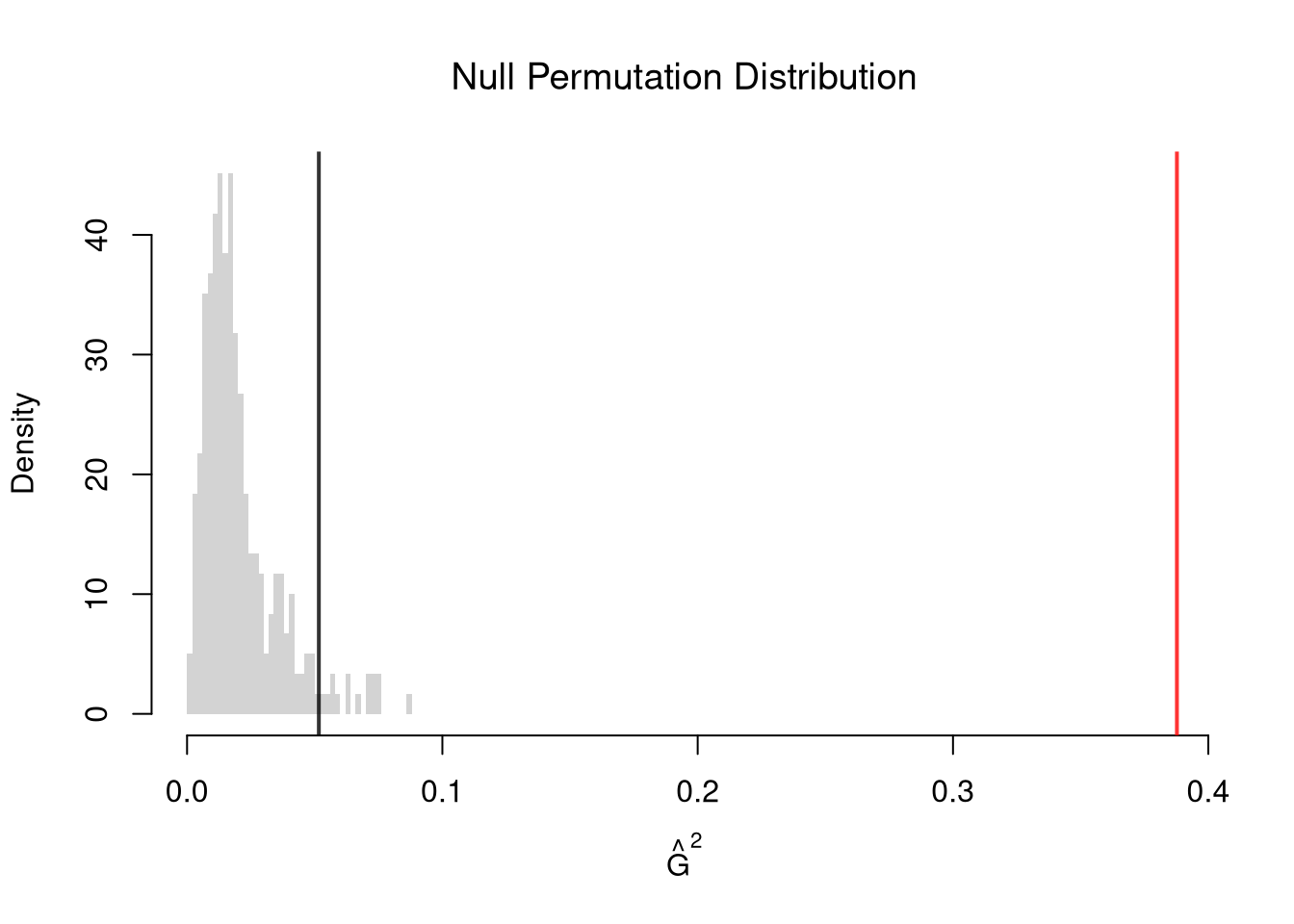
To impose \(H_{0}\), we shuffle \(\hat{x}_{i}\) across observations, as in the permutation test for correlation. Each permutation refits LOESS and recomputes \(\hat{G}^2\). The p-value is the share of permuted \(\hat{G}^2\) at least as large as the observed one. Shuffling makes \(\hat{y}\) unrelated to \(\hat{x}\) in every respect, such as its spread, so it imposes slightly more than \(H_{0}\).

Code
## MAIN EXAMPLE
## Racine's statistic: mean of the squared gradients
## grad_obs defined above
racine_hat <- mean(grad_obs^2)

## Null permutation distribution: shuffle schooling across workers
null_racine <- rep(NA, 299)
for(b in seq_along(null_racine)){
    xy_perm <- xy_hat
    xy_perm[, 'x_hat'] <- sample(xy_perm[, 'x_hat'], replace=FALSE) ## Reshuffle X
    reg_lo_b <- loess(y_hat ~ x_hat, data=xy_perm)
    grad_obs_b <- grad_by_obs(xy_perm, reg_lo_b)
    null_racine[b] <- mean(grad_obs_b^2)
}
perm_cut <- quantile(null_racine, probs=0.95)

## Plot the null distribution, extending the axis to the observed statistic
hist(null_racine, breaks=50,
    border=NA, freq=FALSE,
    xlim=range(c(null_racine, racine_hat)),
    xlab=expression(hat(G)^2),
    main=NA)
title('Null Permutation Distribution', font.main=1)
abline(v=racine_hat, col=rgb(1, 0, 0, .8), lwd=2) # observed statistic
abline(v=perm_cut, col=rgb(0, 0, 0, .8), lwd=2)   # 95% permutation cutoff

Code

## One-sided p-value: P(permuted statistic >= observed statistic)
p_racine <- mean(null_racine >= racine_hat)

cat('Observed statistic: ', round(racine_hat, 3), '\n')
## Observed statistic:  0.388
cat('95% cutoff:         ', round(perm_cut, 3), '\n')
## 95% cutoff:          0.052
cat('Permutation p-value:', p_racine, '\n')
## Permutation p-value: 0
# The observed statistic, about 0.39, is far above the 95% cutoff of about 0.05.
# None of the 299 permuted values is as large, so the p-value is 0.
# That only says the p-value is probably below about 3/299, or 0.01.
# Both tests reject: about 99 percent of workers have a positive gradient.
# So little cancels.

If most gradients share a sign, little cancels, so this test and the test of the mean gradient tend to agree.

17.6 Exercises

  1. Comment the script you wrote for this chapter, then restart R and check that it runs from a clean session, then check the script with AI as explained in Working with AI. Write three sentences from memory on the main statistical idea of this chapter, and ask the assistant what is wrong, vague, or missing. Finish with your own questions about whatever you found hardest.

  2. Using the USArrests dataset, fit a loess regression of Murder on UrbanPop with span = 0.6. Compute the finite-difference gradients \(\hat{b}_{1}(x)\) and report their mean and standard deviation. Compare these to the OLS slope \(\hat{b}_{1}\) from a simple linear regression.

  3. Explain the difference between the gradient at the mean and the mean of the gradients. Why are the two equal for a simple linear regression? Describe a relationship between wages and schooling for which the mean of the gradients is larger than the gradient at the mean.

  4. Using the Wages1 dataset and the default-span loess fit from this chapter, recompute the gradient at the mean, \(\hat{b}_{1}(x=\hat{m}_{X})\), as a finite difference with \(d=0.2\) and with \(d=2\) instead of \(d=1\). How much does it change, and how does the fitted curve near \(\hat{m}_{X}\) explain the change?

  5. Using the loess fit from Exercise 2, compute the gradient at each observation with grad_by_obs(), and bootstrap the standard error of the mean gradient with \(B = 299\) replicates. Test whether the mean gradient differs from zero.

Further Reading

Recall

We used LOESS to reduce bias at the edges of the data and to avoid small samples where the data are sparse. We compared its fit with the line and the regressogram, both in sample and with cross-validation. We then summarized and tested the gradients of a LOESS fit to the Wages1 data. At \(x=15\), the locally constant window mean of about \(6.29\) fell far below the grouped mean of \(8.38\), while a line through the same window predicted about \(8.24\). The small worked example with \(\hat{y}^{\mathrm{pred}}(11.5)=9.2\) and \(\hat{y}^{\mathrm{pred}}(12.5)=10.4\) gave a finite-difference gradient \(\hat{b}_{1}(12)=1.2\) dollars per year of schooling, and the gradient-vector example \((0.4, 0.8, 1.2, 0.9, 0.3)\) at \(x=(8, 10, 12, 14, 16)\) showed the gradient at the mean (\(1.2\)) and the mean of the gradients (\(0.72\)) diverging when the relationship bends. The mean gradient of the LOESS fit, about \(0.58\) dollars per year of schooling, had a bootstrap standard error of about \(0.047\) and a \(\hat{t}\)-statistic of about \(12\), while the gradient at the mean, about \(0.24\), had a 95% confidence interval that included zero. Racine’s statistic \(\hat{G}^2\), about \(0.39\), was far above the \(95\%\) permutation cutoff of about \(0.05\), so we rejected that all gradients are zero.

Adamson, Jordan. 2021. “The Scope of Political Jurisdictions and Violence: Theory and Evidence from Africa.” Public Choice 186 (3): 467–90. https://doi.org/10.1007/s11127-019-00763-8.
Adamson, Jordan. 2025. “Trade and the Rise of Ancient Greek City-States.” Journal of Economic Behavior & Organization 235: 107035. https://doi.org/10.1016/j.jebo.2025.107035.
Chaudhuri, Probal, and J. S. Marron. 1999. “SiZer for Exploration of Structures in Curves.” Journal of the American Statistical Association 94 (447): 807–23. https://doi.org/10.1080/01621459.1999.10474186.
Cleveland, William S. 1979. “Robust Locally Weighted Regression and Smoothing Scatterplots.” Journal of the American Statistical Association 74 (368): 829–36. https://doi.org/10.1080/01621459.1979.10481038.
Cleveland, William S., Susan J. Devlin, and Eric Grosse. 1988. “Regression by Local Fitting: Methods, Properties, and Computational Algorithms.” Journal of Econometrics 37 (1): 87–114. https://doi.org/https://doi.org/10.1016/0304-4076(88)90077-2.
Doksum, Kjell, and Alexander Samarov. 1995. “Nonparametric Estimation of Global Functionals and a Measure of the Explanatory Power of Covariates in Regression.” The Annals of Statistics 23 (5): 1443–73. https://doi.org/10.1214/aos/1176324307.
Hansen, Bruce E. 2022. Econometrics. Princeton University Press. https://www.ssc.wisc.edu/~bhansen/econometrics/.
Härdle, W., and E. Mammen. 1993. “Comparing Nonparametric Versus Parametric Regression Fits.” The Annals of Statistics 21 (4): 1926–47. https://doi.org/10.1214/aos/1176349403.
Henderson, D. J., and C. F. Parmeter. 2015. Applied Nonparametric Econometrics. Applied Nonparametric Econometrics. Cambridge University Press. https://www.the-smooth-operators.com/.
Henderson, Daniel J., Subal C. Kumbhakar, and Christopher F. Parmeter. 2012. “A Simple Method to Visualize Results in Nonlinear Regression Models.” Economics Letters 117 (3): 578–81. https://doi.org/10.1016/j.econlet.2012.07.040.
Mullainathan, Sendhil, and Jann Spiess. 2017. “Machine Learning: An Applied Econometric Approach.” Journal of Economic Perspectives 31 (2): 87–106. https://doi.org/10.1257/jep.31.2.87.
Racine, Jeff. 1997. “Consistent Significance Testing for Nonparametric Regression.” Journal of Business & Economic Statistics 15 (3): 369–78. https://doi.org/10.1080/07350015.1997.10524714.
Racine, Jeffrey S. 2019. An Introduction to the Advanced Theory and Practice of Nonparametric Econometrics: A Replicable Approach Using r. Cambridge University Press. https://doi.org/10.1017/9781108649841.